D Appendix Chapter 4
D.1 Supplemental figures 4.1
Figure D.1: (a) Hysteresis effect in categorization performance for non-identifiable morph series. (b) Adaptation effect in categorization performance for non-identifiable morph series. Note. In the interactive version of this document, hover over the data points to see the related stimuli as well as the exact value and the number of trials related to each data point.
Figure D.2: (a) Hysteresis effect in discrimination performance in case of the non-identifiable morph series. (b) No evidence for adaptation in discrimination performance. Note. In the interactive version of this document, hover over the data points to see the exact value and the number of trials related to each data point.
Figure D.3: (a) Hysteresis effect in perceived similarity in case of non-identifiable morph series. (b) Inconclusive evidence for adaptation effect in perceived similarity. Note. In the interactive version of this document, hover over the data points to see the exact value and the number of trials related to each data point.
D.2 Supplemental figures 4.2
Figure D.4: Categorization performance for the first and the second categorization block per morph series. Note. In the interactive version of this document, hover over the data points to see the related stimuli as well as the exact value and the number of trials related to each data point.
Figure D.5: (a) Hysteresis effect on categorization performance. (b) Adaptation effect on categorization performance. Note. In the interactive version of this document, hover over the data points to see the related stimuli as well as the exact value and the number of trials related to each data point.
Figure D.6: Different representation of adaptation effect on categorization performance. Note. In the interactive version of this document, hover over the data points to see the related stimuli as well as the exact value and the number of trials related to each data point.
Figure D.7: Hysteresis (a) and adaptation (b) effect for the first (cat1) and second (cat2) categorization task separately. Note. In the interactive version of this document, hover over the data points to see the related stimuli as well as the exact value and the number of trials related to each data point.
Figure D.8: (a) Individual slope estimates for the effect of the current morph stimulus level based on a Bayesian multilevel logistic regression model. (b) Correlation between individual stimulus and hysteresis effect estimates. (c) Correlation between individual stimulus and adaptation effect estimates. Note. Black dots and grey lines indicate the median and 95% highest density continuous interval per individual. The black and the blue line indicate the null value and the average median across participants respectively. In the interactive version of this document, hover over the data points to see the exact values for each individual participant.
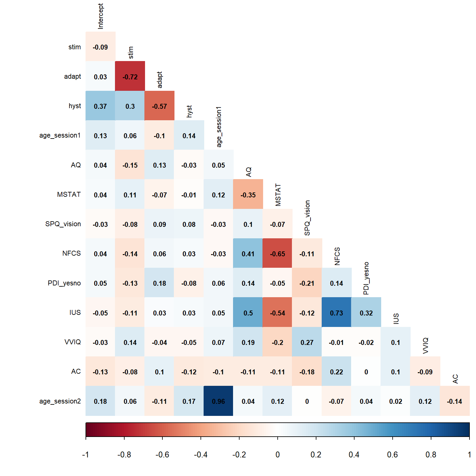
Figure D.9: Correlations between behavioral indices and questionnaires. Abbreviations: ‘stim’ = estimated effect of current morph level, ‘adapt’ = estimated effect of previous morph level, ‘hyst’ = estimated effect of previous percept, ‘AQ’ = Autism Quotient, ‘MSTAT’ = Multiple Stimulus Types Ambiguity Tolerance Scale-II, ‘SPQ_vision’ = vision subscale of the Sensory Perception Quotient, ‘NFCS’ = Need for Closure Scale, ‘PDI_yesno’ = Peters’ Delusional Inventory (yes-no responses), ‘IUS’ = Intolerance of Uncertainty Scale, ‘VVIQ’ = Vividness of Visual Imagery Questionnaire, ‘AC’ = attention check.
D.3 Methodological information 4.2
The study consisted of two separate research sessions. In the first session (N = 216), most of the questionnaire data (except for the Autism Quotient) was collected. The second session (N = 209) included the categorization task and the Autism Quotient questionnaire. 131 participated in both sessions. In what follows we will only detail the information for the second session.
Participants: 209 first-year psychology students from KU Leuven participated in the second part of the study (87.08% female, age between 17 and 28, mean age = 18.65, sd age = 1.44).
Material: Stimuli were a subset of two series of non-identifiable morph figures used in the study described in 3 (based on stimuli from Op de Beeck et al., 2003a). More specifically, when we define the extremes of the series containing 11 stimuli as -5 and 5, levels -5, -3, -1, 0, 1, 3, and 5 were used.
The experiment itself was written in Python 3 and run on Windows computers with TFT screens of 21,5".
Procedure: Students participated in groups. After giving informed consent and completing some demographical questions, each participant completed the categorization task for both non-identifiable morph series (a separate block for each morph series) two times. The order of the morph series was randomized across but fixed within participants. Afterwards, participants completed the Autism Quotient questionnaire and completed a third and fourth block of categorization trials for each morph series (in the same order as the first time).
At the start of the first categorization block, participants completed four example trials with a separate morph series (see C). Before the start of each block of categorization trials, participants were shown four ‘clear’ exemplars per category, to give them an idea of the categories. In the middle of each block, the response buttons switched meaning. Participants were informed about this switch with new instructions and were reminded of the current meaning of the buttons on each response screen.
Each trial in the categorization task consisted of (a) the presentation of a fixation cross (500 ms); (b) the presentation of the stimulus (300 ms); (c) a response screen reminding participants which arrow key to press for category A and which for category ; and (d) a blank interval (400 ms). In other words, the interstimulus interval had a duration of 900 ms (400 ms blank screen and 500 ms fixation cross). The exact position of the stimuli was jittered (from -20 to 20 on both x and y axes) to prevent focus on local feature changes only. As we were interested in the effect of the previous stimulus level on the current percept, we made sure that all possible stimulus pairs were repeated at least twice in each block of trials. The presentation order of these stimulus pairs within each block was randomized. Each block contained 392 stimuli, so participants were presented with 1568 stimuli in total (2 morph series, 2 blocks per morph series).
In the interactive version of this document, you find screen recordings of some trials of each task in this study.
Availability study materials: The data and materials for this project are available on Open Science Framework: https://doi.org/10.17605/OSF.IO/56X8J.
D.4 Supplemental Figures 4.3
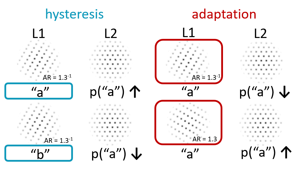
Figure D.10: Illustration of attractive and repulsive context effects in dot lattices. Left: attraction effect (hysteresis). When the first lattice (L1) is perceived as orientation a, the probability that the second lattice (L2) will be perceived as orientation a is higher than when L1 was interpreted as orientation b. Right: repulsion effect (adaptation). When strong support for orientation a is present in L1, the probability that L2 will be perceived as a orientation a is lower than when L1 had less support for orientation a.
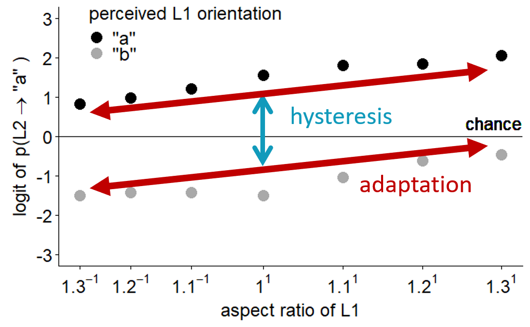
Figure D.11: Expected average effects of hysteresis and adaptation on the perception of multistable dot lattices, based on the study of Schwiedrzik et al. (2014). Vertical separation of the two lines reflects the size of the perceptual hysteresis effect, the slope of both lines reflects the size of the perceptual adaptation effect.
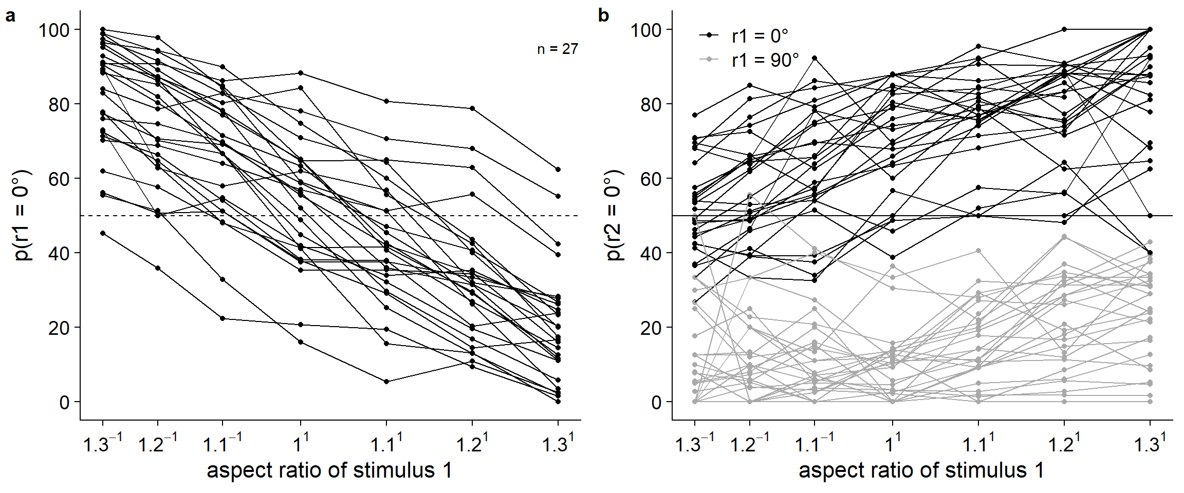
Figure D.12: (a) Mean individual responses to the first stimulus dependent on aspect ratio (probability). The probability of responding 0° to the first stimulus decreases with aspect ratio (d0/d90). The value of aspect ratio increases with increasing distance in the 0°-orientation, leading to more 90° responses. (b) Mean individual responses to the second stimulus dependent on aspect ratio (probability). The probability of responding 0° to the second stimulus increases with aspect ratio (d0/d90; i.e., adaptation effect), and increases when the first stimulus was perceived as 0° rather than 90° (i.e., hysteresis effect).
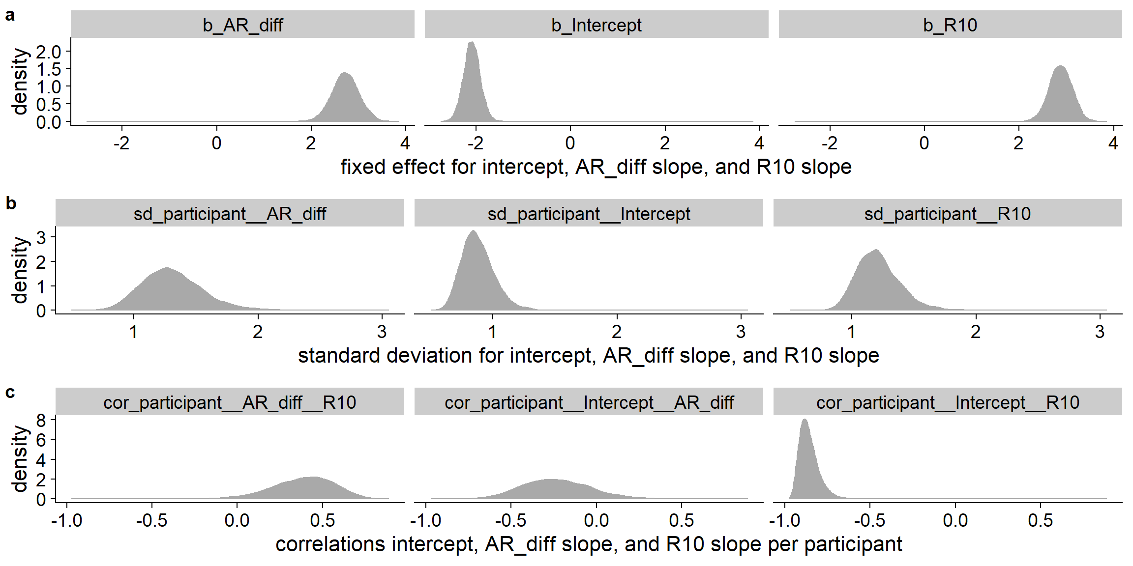
Figure D.13: Posterior distributions of fixed effects, standard deviation of random effects, and the correlation between the random effects for the model of perceived L2 orientation.
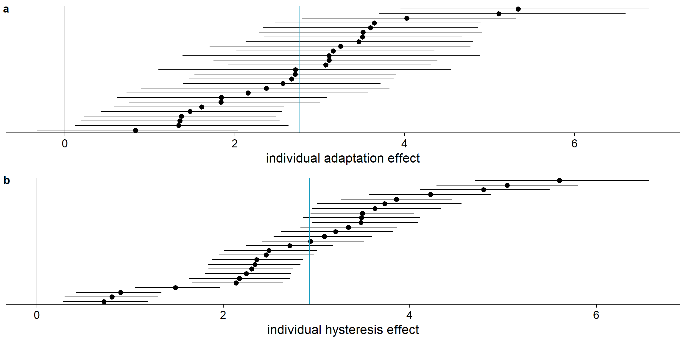
Figure D.14: Slopes for the effect of aspect ratio and perceived L1 orientation on perceiving the 0° orientation in L2 per participant. Median and 95% highest density continuous intervals are shown. The blue line indicates the average median slope across participants. The black line indicates a slope of zero.
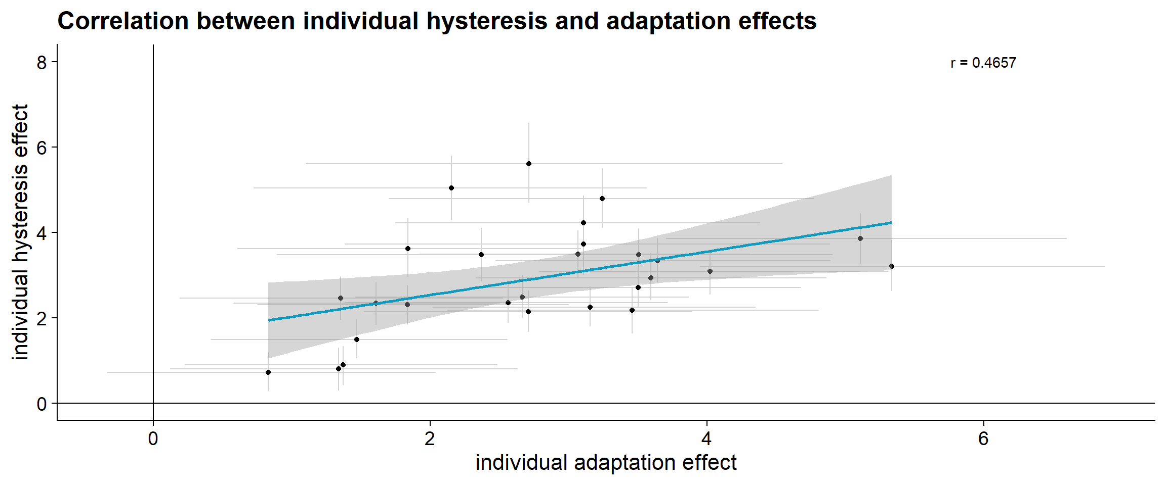
Figure D.15: Correlation between individual slopes for the effect of aspect ratio and perceived L1 orientation on perceiving the 0° orientation in L2. Median and 95% highest density continuous intervals are shown. The blue lines indicate a slope of zero.
D.5 Supplemental information 4.3
As the study of Schwiedrzik et al. (2014) did not include a measure of absolute orientation bias, we do not have any data on the relation between absolute bias with the hysteresis and adaptation effects yet. We do however have some pilot results from a science communication event, where 31 participants did 10 to 60 trials to find out their own orientation bias. These pilot data (Figure D.16) hint at diversity in both the direction of this bias as well as the strength of the bias, although more and more controlled data collection is needed to evaluate this properly. In addition, these pilot data show that at least some consistency in the direction and strength of the bias can be found between different blocks when participants completed more than one block of ten trials.
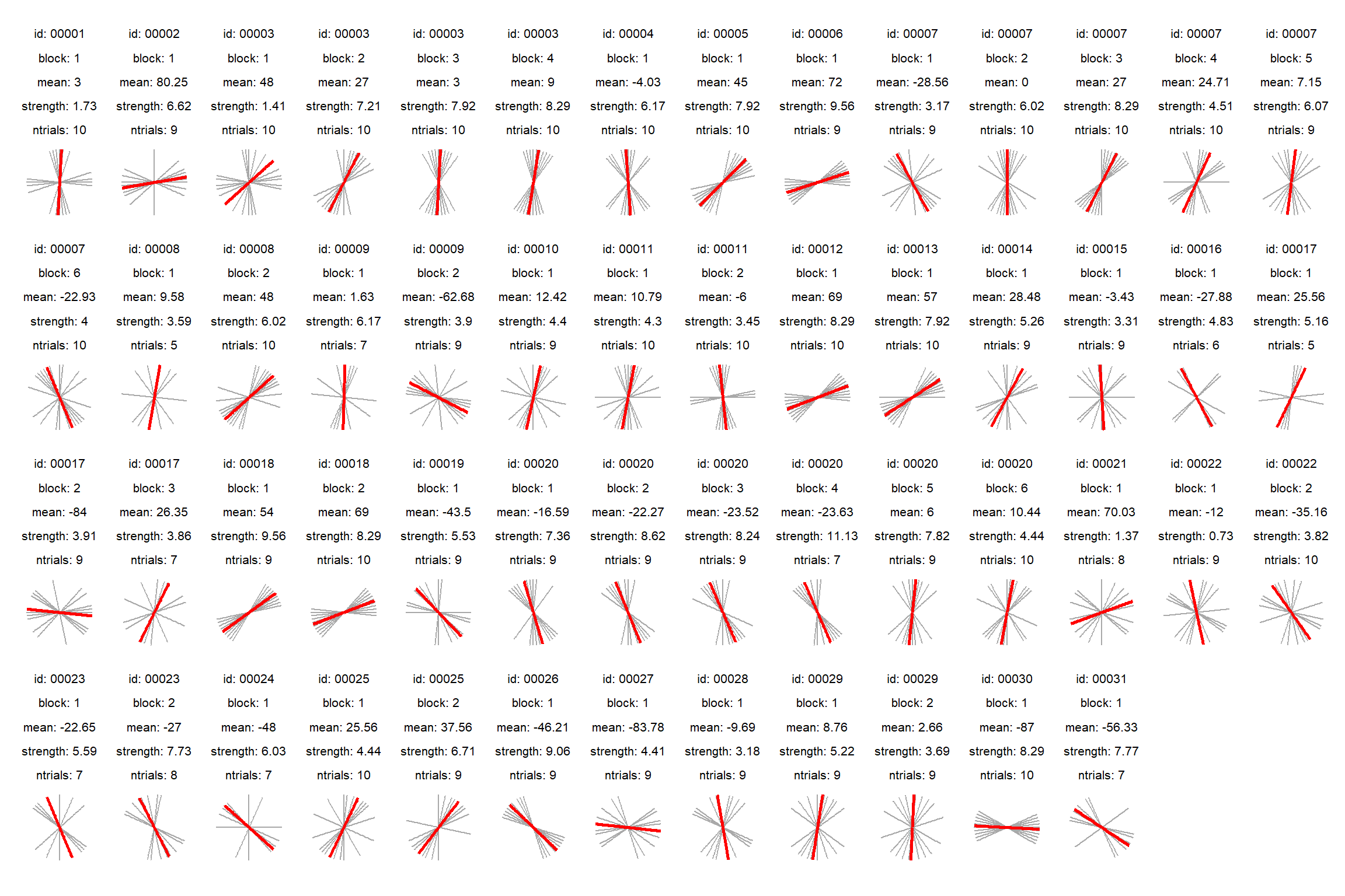
Figure D.16: Visual representation of the absolute orientation bias of an individual per block of ten trials, corrected for implausible 90° responses.
In the interactive version of this document, you find screen recordings of some trials of each proposed task in this study.
D.6 Supplemental videos 4.4
In the interactive version of this document, you find screen recordings of some trials of each proposed additional task (instructions not included).