Appendix C — Efficient Bayesian observer model of hysteresis and adaptation

C.1 R packages used

As indicated in the Methods section, for all our analyses we used R (Version 4.0.4; R Core Team, 2021) and the R-packages BayesFactor (Version 0.9.12.4.2; Morey & Rouder, 2018), brms (Version 2.16.1; Bürkner, 2017, 2018, 2021), coda (Version 0.19.4; Plummer et al., 2006), cowplot (Version 1.1.1; Wilke, 2020), devtools (Version 2.4.4; Wickham, Hester, et al., 2021), doParallel (Version 1.0.17; Corporation & Weston, 2020), dplyr (Version 1.0.10; Wickham, François, et al., 2022), ellipse (Version 0.4.2; Murdoch & Chow, 2020), forcats (Version 0.5.2; Wickham, 2022), foreach (Version 1.5.2; Microsoft & Weston, 2020), GGally (Version 2.1.2; Schloerke et al., 2021), ggdist (Version 3.0.0; Kay, 2021a), ggforce (Version 0.3.3; Pedersen, 2021), ggnewscale (Version 0.4.8; Campitelli, 2022), ggplot2 (Version 3.3.6; Wickham, 2016), ggstance (Version 0.3.5; Henry et al., 2020), glue (Version 1.6.2; Hester & Bryan, 2022), gmm (Version 1.7; Chaussé, 2010), here (Version 1.0.1; Müller, 2020), iterators (Version 1.0.14; Analytics & Weston, 2020), kableExtra (Version 1.3.4; Zhu, 2021), knitr (Version 1.39; Xie, 2015), lubridate (Version 1.8.0; Grolemund & Wickham, 2011), MASS (Version 7.3.53; Venables & Ripley, 2002), Matrix (Version 1.3.2; Bates & Maechler, 2021), mvtnorm (Version 1.1.3; Genz & Bretz, 2009; Wilhelm & G, 2022), papaja (Version 0.1.1; Aust & Barth, 2022), patchwork (Version 1.1.2; Pedersen, 2022), purrr (Version 0.3.4; Henry & Wickham, 2020), Rcpp (Eddelbuettel & Balamuta, 2018; Version 1.0.9; Eddelbuettel & François, 2011), readr (Version 2.1.2; Wickham, Hester, et al., 2022), rstan (Version 2.21.2; Stan Development Team, 2020a), sandwich (Zeileis, 2004, 2006; Version 3.0.2; Zeileis et al., 2020), StanHeaders (Version 2.21.0.7; Stan Development Team, 2020b), stringr (Version 1.4.0; Wickham, 2019), tibble (Version 3.1.8; Müller & Wickham, 2022), tidybayes (Version 3.0.1; Kay, 2021b), tidyr (Version 1.2.1; Wickham & Girlich, 2022), tidyverse (Version 1.3.2; Wickham et al., 2019), tinylabels (Version 0.2.3; Barth, 2022), tmvtnorm (Version 1.5; Wilhelm & G, 2022), truncnorm (Mersmann et al., 2018), and usethis (Version 2.1.6; Wickham, Bryan, et al., 2021).

C.2 Visualization of prior, likelihood, and posterior distributions for one trial

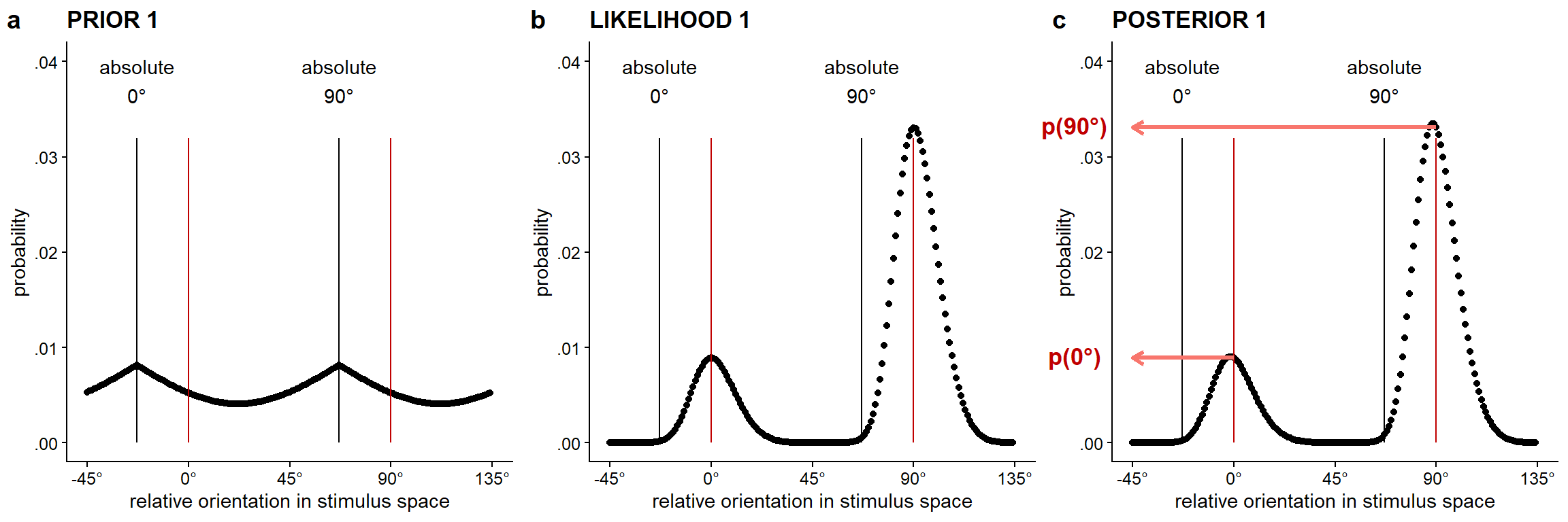
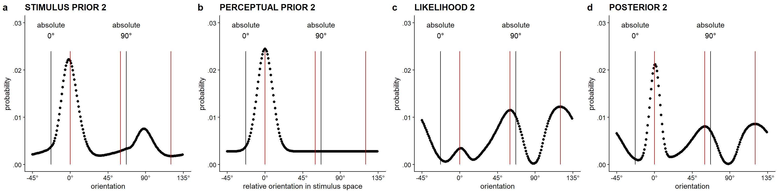
Figure C.1 visualizes the prior, likelihood, and posterior distributions for the first lattice in a single trial of the dot lattices paradigm, given a model with a prior stimulus distribution incorporating the more frequent occurrence of cardinal compared to oblique orientations. Figure C.2 visualizes the prior, likelihood, and posterior distributions for the second lattice in a single trial of the dot lattices paradigm, given the same natural stimulus distribution for the prior of the first lattice.

Figure C.1: (a) Natural stimulus prior for the first lattice, defined by the formula: \(p(\theta) = c_0(2 - |sin (\theta)|)\), in which \(\theta\) represents the orientation value and \(c_0\) the normalizing constant. (b) Example of likelihood 1 defined in the stimulus space, for a first lattice with an absolute lattice orientation of 23° and AR = 1.3^-1, which favors the relative 0° orientation. (c) Posterior distribution for the first lattice. Based on the difference in height of the peaks for the relative 0° and 90° orientation, i.e., p(0°) and p(90°), the probability of a} 0° or 90° response can be determined. *Note.* The red vertical lines in the graph are placed at the two dominant relative 0° and 90° orientations in the lattice. The black vertical lines label the absolute 0° and 90° orientations.

Figure C.2: (a) Stimulus prior for the second lattice given a first lattice with an absolute lattice orientation of 23° and with AR = 1.3^-1, which favors the relative 0° orientation. (b) Perceptual prior for the second lattice, given the relative 0° orientation was perceived in the first lattice. (c) Likelihood distribution defined in the stimulus space for the second lattice. This distribution is influenced by the stimulus prior for the second lattice (and hence the aspect ratio of the first lattice) via the stimulus-to-sensory mapping. (d) Posterior distribution for the second lattice, combining perceptual prior and likelihood for the second lattice. Based on the difference in height of the peaks for the relative 0°, 60°, and 120° orientation, the probability of a 0°, 60°, or 120° response can be determined. *Note.* The red vertical lines in the graph are placed at the three dominant relative 0°, 60°, and 120° orientations in the lattice. The black vertical lines label the absolute 0° and 90° orientations.

C.3 Supplementary Figures related to the section “Approximation of average attractive and repulsive temporal context effects”

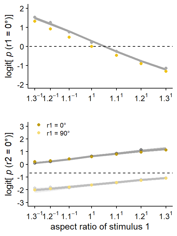
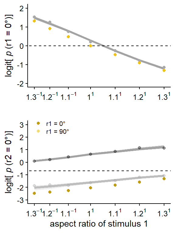
Figure C.3 visualizes the logit probability of perceiving the relative 0° orientation based on efficient Bayesian observer model with a natural stimulus distribution prior for the first lattice. Figure C.4 visualizes the logit probability of perceiving the relative 0° orientation based on efficient Bayesian observer model without a perceptual prior and with a more extreme weighting of the previous stimulus evidence than in Figure 5.4b.

Figure C.3: Visualization of the logit probability to perceive the relative 0° orientation in (a) the first lattice and (b) the second lattice, based on an efficient Bayesian observer model with a natural stimulus distribution prior for the first lattice and the following parameters: \(c\)_stim = 5, \(\kappa\)_stimL1 = 20, \(\kappa\)_sensL1 = 20, \(\kappa\)_stimL2 = 20, \(\kappa\)_sensL2 = 18, \(\kappa\)_percL1 = 10, \(w\)~stimL1 = 0.60, and \(w\)_percL1 = 0.50. The yellow dots indicate the probabilities based on the model. The behavioral results and the estimated effects based on the behavioral results of Van Geert et al. (2022), averaged across participants, are indicated in grey.

Figure C.4: Visualization of the logit probability to perceive the relative 0° orientation in (a) the first lattice and (b) the second lattice, based on an efficient Bayesian observer model without a perceptual prior for the second lattice, a flat prior distribution for the first lattice, and the following parameters: \(c\)_stim = 5, \(\kappa\)_stimL1 = 20, \(\kappa\)_sensL1 = 20, \(\kappa\)_stimL2 = 20, \(\kappa\)_sensL2 = 18, \(\kappa\)_percL1 = 10, \(w\)_stimL1 = 1, and \(w\)_percL1 = 0. The blue dots indicate the probabilities based on the model. The behavioral results and the estimated effects based on the behavioral results of Van Geert et al. (2022), averaged across participants, are indicated in grey.

C.4 Supplementary information concerning Bayesian analyses of interindividual variation in simulation data

We estimated individual hysteresis and adaptation effects using a Bayesian multilevel binomial regression model predicting the percept of the second lattice, with aspect ratio of the first lattice (\(AR\)) and the percept of the first lattice (\(R10\)) as fixed and random effects. To estimate the direct proximity effect (i.e., the direct effect of aspect ratio on perception of the first lattice), we used a Bayesian multilevel binomial regression model predicting the percept of the first lattice, with aspect ratio of the first lattice (\(AR\)) as fixed and random effect.

The model for the first lattice included fixed and individual random effects for aspect ratio AR (i.e., proximity effect), and individual random intercepts. This model can be formulated as follows: \[ freq(r1 = 0^{\circ}) | trials(n) \sim Intercept + AR + (Intercept + AR \; | \; participant).\] To determine the size of the proximity effect, we used the individual estimates for the effect of the aspect ratio of the first lattice on the percept of the first lattice.

The model for the second lattice thus included fixed and individual random effects for percept in the first lattice R10 (i.e., hysteresis effect) as well as aspect ratio in the first lattice AR (i.e., adaptation effect), and individual random intercepts. This model can be formulated as follows: \[ freq(r2 = 0^{\circ}) | trials(n) \sim Intercept + AR + R10 + (Intercept + AR + R10 \; | \; participant).\] To determine the size of the hysteresis effect, we used the individual estimates for the effect of the percept of the first lattice on the percept of the second lattice. To determine the size of the adaptation effect, we used the individual estimates for the effect of aspect ratio of the first lattice on the percept of the second lattice. To have an estimate of the strength of the correlation between the size of individuals’ hysteresis and adaptation effects, we report the mean and 95% HDCI for the correlation between estimated individual hysteresis and adaptation effects, based on the full model described above.

In both the model for the first and for the second lattice, centered aspect ratio was used, which means that a value of zero corresponds to an aspect ratio of 1, a value of 1.1^-1 -1 (i.e., \(\approx\) -0.09) corresponds to 1.1^-1, and a value of 1.1¹ -1 (i.e., 0.10) to an aspect ratio of 1.1.

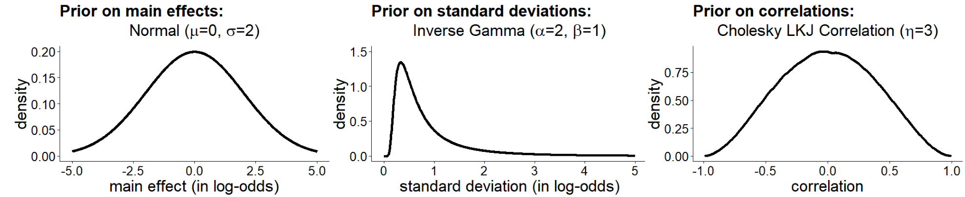
Figure C.5 visualizes the priors we specified for the fixed effects, for the standard deviation of the random effects, and for the correlation matrix.

Figure C.5: Illustration of priors used in the model predicting the percept of L1 and L2. Reprinted from Van Geert et al. (2022).

We fitted these models of perceived L1 and perceived L2 orientation using brms (Bürkner, 2017, 2018). We used 4 chains with 20000 iterations each with the default number of warmup iterations per chain. For any other sampling specifications we used the default settings. For further details on these analyses and those for calculating the correlation between individuals’ proximity, hysteresis, and adaptation estimates, please consult Van Geert et al. (2022).

C.5 Supplementary Figure concerning interindividual variation in proximity, hysteresis, and adaptation

Figure C.6 visualizes the correlation of estimated individual hysteresis and adaptation effects concerning the second lattice with estimated individual proximity effects concerning the first lattice for the empirical data collected in Van Geert et al. (2022) and for the simulation results.

Figure C.6: Correlation of estimated individual hysteresis and adaptation effects concerning the second lattice with estimated individual proximity effects concerning the first lattice for (a) the empirical data collected in Van Geert et al. (2022) and (b) the simulation results.

C.6 Shiny application

Figure C.7 shows the Shiny application to visualize the prior, likelihood, and posterior distributions for one trial under different parameter settings.

Figure C.7: A Shiny application to visualize the prior, likelihood, and posterior distributions for one trial under different parameter settings. Click the link to try out the application.