6 Towards the most prägnant Gestalt: Leveling and sharpening as contextually dependent adaptive strategies
Van Geert*, E., Frérart*, L., & Wagemans, J. (under review). Towards the most prägnant Gestalt: Leveling and sharpening as contextually dependent adaptive strategies. Preprint available from https://doi.org/10.31234/osf.io/t3bzw
* Eline Van Geert and Liesse Frérart contributed equally to this work.
Preprint Materials, data, and code
Abstract
Gestalt psychologists posited that we always organize our visual input in the best way possible under the given conditions. Both weakening or removing unnecessary details (i.e., leveling) and exaggerating distinctive features (i.e., sharpening) can contribute to achieve a better organization. When will a feature be leveled or sharpened, however? We investigated whether the importance of a feature for discrimination among alternatives influences which organizational tendency occurs. Participants were simultaneously presented with four figures composed of simple geometrical shapes, and asked to reconstruct one of these figures in such a way that another participant would be able to recognize it among the alternatives. The four figures differed either qualitatively or only quantitatively (i.e., far or close context). Regarding quantitative differences, two feature dimensions were varied, with one manifesting a wider range of variability across the alternatives than the other. In case of a smaller variability range, the target figure was either at the extreme of the range or had an in-between value. As expected, the results indicated that sharpening occurred more often for the feature with an extreme value, for the feature exhibiting more variability, and for the features of figures presented in the close context, than for the feature with a non-extreme value, exhibiting less variability, or in the far context. In line with Metzger’s (1941) definition of prägnant Gestalts, the essence of a Gestalt is context-dependent, and this will influence whether leveling or sharpening of a feature will lead to the best organization in the specific context.
Context dependence of leveling and sharpening
6.1 Introduction
In the beginning of the 20th century, the Gestalt psychologist Max Wertheimer coined the law of Prägnanz der Gestalt or the law of a tendency towards establishing clear, simple Gestalts or experienced organizations (Schumann, 1914). The best-known English definition of the Prägnanz tendency was given by Koffka (1935, p. 110): “psychological organization will always be as ‘good’ as the prevailing conditions allow”. Prägnanz or goodness of organization is a multifaceted concept (Metzger, 1941; Rausch, 1966; Van Geert & Wagemans, 2023). Rausch (1966) indicated that for an organization to be experienced as ‘good’ or ‘prägnant’, the organization should be experienced as lawful (i.e., non-random). Furthermore, a psychological organization will be ‘better’ when the organization is experienced as autonomous rather than derived, complete rather than disturbed, simple of structure rather than complicated of structure, element rich rather than meager, expressive rather than lacking expressiveness, and meaningful rather than meaningless (Rausch, 1966; cf. also Van Geert & Wagemans, 2023). These specifications of Prägnanz indicate that the goodness of an organization can increase with increasing lawfulness and regularity as well as with increasing intricacy and complexity (Rausch, 1966; Van Geert & Wagemans, 2023). Two main aspects are important to fully understand the meaning of Prägnanz, according to Metzger (1941). On the one hand, prägnant organizations show an outstanding and consequently persistent figural order (i.e., unity, regularity). On the other hand, psychological organizations are experienced as prägnant when they are completely specified structures in which the essence of the organization is most pure and compelling. Thus, both form-related and content-related aspects may play a role in the goodness of a psychological organization (Metzger, 1941; Rausch, 1966; Van Geert & Wagemans, 2023).
Taking the tendency towards better psychological organizations as a starting point, how can we clarify the incoming stimulation to come to a better psychological organization? Koffka (1935) specified two variants of the tendency towards prägnant Gestalts: either as much or as little will happen as the prevailing conditions allow. The former is referred to as maximum simplicity or the simplicity of perfect articulation, the latter as minimum simplicity or the simplicity of uniformity. For example, given a figure with slightly unequal tips as the middle one in Figure 6.1, one can either downplay this inequality and make the figure more symmetric (i.e., minimum simplicity, leveling), or one can intensify this inequality and make the figure more asymmetric (i.e., maximum simplicity, sharpening).
Importantly, which organization will be experienced as ‘better’ will depend on the prevailing conditions: the incoming stimulation, the perceiving individual, and the context in which the stimulation is encountered (Koffka, 1935; Van Geert & Wagemans, 2023). In this example, the experienced organization is compared to an internal reference (e.g., a figure with equal, symmetrical tips). The differences in comparison to this internal reference can be diminished (i.e., leveling), or they can be exaggerated (i.e., sharpening; Van Geert & Wagemans, 2023). However, if the same figure would be presented under different conditions, for example, in spatial or temporal proximity to similar figures with either more or less equal tips, a local reference may be used. That is, the original figure may be evaluated in the context of these other figures in the display (cf. Figure 6.1).
Although Koffka (1935) viewed minimum and maximum simplicity (i.e., leveling and sharpening) as alternative tendencies, Arnheim (1986) considered them as antagonistic but complementary tendencies concurrently present in every perceptual event. That is possible because perception is inherently multidimensional. In our example, we can not only evaluate the figure on the equality of its tips, but we can also evaluate the size of the figures, the thickness or luminance of the lines, etc. (cf. Figure 6.2). To clarify the incoming stimulation, tension-reducing tendencies (i.e., leveling, simplification, minimum simplicity) will increase the experienced regularity in the figure and remove distracting, unessential details, while tension-enhancing tendencies (i.e., sharpening, complication, maximum simplicity) will intensify the figure’s characteristic features (Arnheim, 1986; Van Geert & Wagemans, 2023). In this way, leveling and sharpening can concurrently contribute to the Prägnanz (clarity) of a Gestalt (Arnheim, 1986; Hubbell, 1940; Köhler, 1951/1993; Van Geert & Wagemans, 2023).
Recent work on consistent, specific false memories for some images from popular iconography confirmed the idea that both leveling and sharpening1 can lead to a better psychological organization (Prasad & Bainbridge, 2022). For example, Pikachu (from the Pokémon franchise) is consistently remembered to have a yellow tail with a black tip (i.e., adding a characteristic feature: Pikachu’s ears have black tails) instead of an almost completely yellow tail with a patch of brown at the base (i.e., removing an unessential detail: the patch of brown is experienced as unessential).
Importantly, leveling and sharpening tendencies towards the best psychological organization given the prevailing conditions can occur at two levels (Hüppe, 1984; Van Geert & Wagemans, 2023). Primary Prägnanz tendencies occur from the stimulus to the percept: when we perceive a stimulus, our percept already deviates from the stimulus, and this deviation is unconscious to the observer (Hüppe, 1984; Van Geert & Wagemans, 2023). Secondary Prägnanz tendencies on the other hand operate at the level of experience: although one may be able to perceptually discriminate the experienced organization from the reference, one may cognitively evaluate the organization in relation to the reference (Hüppe, 1984; Van Geert & Wagemans, 2023; Wertheimer, 1923). In our example, one may be able to visually perceive the difference between the figure with equal and slightly unequal tips, but one may cognitively evaluate the slightly unequal figure as “almost equal” (i.e., secondary leveling). This evaluation can sometimes occur consciously (Hüppe, 1984).
Furthermore, these secondary leveling and sharpening tendencies can also be voluntarily applied as communicative strategies. This is the case, for example, in the work of artists, who will go beyond the physical stimulation they receive in the direction of Prägnanz, to more purely and compellingly represent an essence (Arnheim, 1975; Metzger, 1941). Scott McCloud (1993) pointed to the use of leveling and sharpening strategies in cartoons in his work ‘Understanding comics’. He described cartooning as a form of ‘amplification through simplification’: cartooning is said to be not so much about eliminating details but about focusing on specific details, and this to strip an image down to its essential meaning (McCloud, 1993, p. 30). This idea corresponds closely to the idea of leveling and sharpening as co-occurring tendencies to come to a better psychological organization (Arnheim, 1986). Secondary Prägnanz tendencies are not completely independent of primary Prägnanz tendencies, however: to be able to consciously evaluate and/or manipulate the closeness of an experienced organization to a reference, the organization first needs to be perceived.
Also in more recent scientific literature on the origin of errors in drawing, this distinction between primary and secondary Prägnanz tendencies comes back. Cohen & Bennett (1997) distinguished four psychological sources for drawing errors: (1) misperception of the object, (2) misperception of the drawing, (3) motor skills, and (4) representational decisions (cf. also Chamberlain & Wagemans, 2016). From a series of drawing experiments isolating different components of the drawing process, Cohen & Bennett (1997) concluded that misperception of the object was most crucial for drawing errors. Also later studies found evidence for the idea that there is close link between internal representations of objects and how they are drawn (Chamberlain & Wagemans, 2016; Cohen, 2005; Fan et al., 2018; Matthews & Adams, 2008). For example, Ostrofsky et al. (2015) and Mitchell et al. (2005) found reliable relations between illusion strength and drawing accuracy. On the other hand, also misperception of the drawing and representational decisions play a role in drawing errors (Chamberlain & Wagemans, 2016; Cohen & Bennett, 1997). Concerning representational decisions, Ostrofsky et al. (2012) found that artists were better at producing recognizable minimal line drawings than non-artists, probably because the artists included more features necessary for object recognition. Also Chamberlain & Wagemans (2016) concluded that artists probably know better which parts of a visual image are crucial, and this is important for later identification of the drawn image. Misperceptions of the object and/or the drawing may here be attributed to primary Prägnanz tendencies leading to deviations from stimulus to percept, while the representational decisions can be related to secondary Prägnanz tendencies.
Given a specific figure, which primary and secondary Prägnanz tendencies will occur? That will depend on the prevailing internal and external conditions (Koffka, 1935). External conditions are created in the receptor organs by the physical stimulation they receive, internal conditions are inherent to the human nervous system, which can be more permanent or more temporary (cf. also Van Geert & Wagemans, 2023). When the external conditions are weak (i.e., limited visibility due to, e.g., low contrast, brief presentation, or small size), primary Prägnanz tendencies will get more room and lead to tangible deviations of the percept compared to the external stimulation (Koffka, 1935). When the external conditions are stronger, primary Prägnanz tendencies will be more constrained, but secondary Prägnanz tendencies can still play an important role in how the organization is experienced.
6.1.1 Empirical evidence for Prägnanz tendencies
Wulf (1922) asked participants to reproduce abstract figures from memory after different time intervals, going from 30 seconds to two months. He found empirical evidence for both leveling (i.e., weakening one or more features of a figure) and sharpening (i.e., exaggerating one or more features of a figure). Allport (1930) conducted a similar study in large groups of children. His findings indicated a tendency towards symmetry, and several changes in the reproductions could be categorized as leveling and sharpening. Fehrer (1935) also noticed leveling and sharpening tendencies in reproductions, but under different conditions: participants were repeatedly exposed to these figures for short periods of time. In addition, she found evidence for related tendencies such as simplification and complication (i.e., the use of fewer or more parts in the reproduction compared to the original), and for tendencies towards symmetry.
Building on Wulf’s (1922) study, Gibson (1929) studied memory reproductions in figures that could be changed in more diverse ways, which made it more difficult to categorize changes as either leveling or sharpening. Similar to Wulf (1922), he found a ‘normalizing’ tendency: when a figure had previously been associated with a familiar object, reproductions of the figure deviated in the direction of this familiar object. We could thus say that the participant’s internal representation of that familiar object served as a reference. Also Granit (1922) found evidence for normalizing tendencies when he asked both children and adults to reproduce figures to which they were exposed very briefly. This normalizing tendency was interpreted by Wulf (1922) as one way in which reproductions can be leveled. Furthermore, Gibson (1929) also described leveling tendencies in comparison to a local reference: when two figures had previously been associated, one figure’s reproduction frequently changed in the direction of the other figure.
Hubbell (1940) asked participants to freely change given geometrical figures until they considered them ‘good’ figures. Different from the above reported studies, in this study by Hubbell (1940) the viewing conditions were not limited. Therefore, this study tapped more into secondary Prägnanz tendencies, while the studies reported above focused on studying primary Prägnanz tendencies. Although a considerable proportion of the figures was simplified (i.e., removing parts), participants most frequently changed the figures in the direction of greater differentiation (i.e., complication, adding parts), but importantly, these changes enhanced the unity and coherence of the original figure. Similar tendencies were found by Wohlfahrt (1932), when he presented participants with abstract line figures in a very small size. Participants’ reproductions showed tendencies towards regularity: their reproductions were more meaningful and complex than the figures from which they originated (i.e., sense making through complication). In sum, the complication of figures (i.e., addition of lines or dots) did not indicate a more complex end result in these studies; by adding lines, simplicity was achieved (Hubbell, 1940).
Also more recent work confirmed biases towards a better psychological organization. Feldman (2000) asked participants to draw a triangle and a quadrilateral, and the produced shapes were biased towards equilateral triangles and squares, respectively. Miller and Gazzaniga (1998) found evidence for false recognition of schema-consistent items in visual scenes (e.g., a beach ball in a beach scene; cf. also Brewer & Treyens (1981) and Roediger III & McDermott (1995) for the same tendency for real scenes and for words, respectively). This can be interpreted as a sharpening tendency in memory (i.e., the beach becomes more ‘beachy’ by adding the ball). Also, some studies reported more false recognition for gist-consistent versus gist-inconsistent pictures (Koutstaal & Schacter, 1997) and for high-frequency compared to low-frequency category exemplars (Seamon et al., 2000). Furthermore, this difference in false recognition rates increased over time (Seamon et al., 2000).
Rosielle & Hite (2009) showed that participants sharpened the small but noticeable difference in size between two or three simultaneously presented simple shapes in their drawings from memory. Also when directly copying the figure, participants showed a sharpening tendency. The authors strongly argued against explaining this sharpening as a conscious strategy (i.e., secondary Prägnanz tendency) in their study, given that almost all participants showed the sharpening tendency in spite of being told repeatedly to draw the stimuli as veridically as possible, and given that expert drawers showed reduced sharpening compared to novices. Rosielle & Hite (2009) named this effect the ‘caricature’ effect in drawing, after the investigations showing better and faster recognition for caricature drawings of faces compared to veridical face drawings, both for familiar and unfamiliar faces (e.g., Lee et al., 2000; Mauro & Kubovy, 1992; Rhodes et al., 1987; Robert, 1999; Stevenage, 1995). Furthermore, Rodríguez et al. (2009) showed that being familiarized with caricature faces during training improved recognition for veridical drawings in a test phase. In addition, caricature effects have also been found for other stimulus categories than faces. Rhodes & McLean (1990) observed that for both experts and non-experts, transformations of bird drawings that increased distinctiveness (i.e., sharpening, caricature) led to faster identification and higher recognition than anticaricatures (i.e., leveling). Furthermore, for experts there was also a caricature advantage, with caricatures of birds in a highly homogeneous and familiar class being identified more quickly than uncaricatured veridical drawings (Rhodes & McLean, 1990).
6.1.2 Conditional dependencies of Prägnanz tendencies
The above described studies indicate that both primary and secondary leveling and sharpening tendencies can occur to clarify an experienced organization, and that this clearer organization can lead to better identification and recognition performance. But when will leveling or sharpening of a particular feature occur? Which tendency will lead to a better psychological organization, will depend on the prevailing conditions (Koffka, 1935; Van Geert & Wagemans, 2023). These can be roughly categorized in stimulus-, person-, and context-level conditions.
Concerning stimulus-level conditions, Allport (1930) indicated that broken lines, acute angles and marked asymmetry are features likely to be sharpened. Goldmeier (1972) coined the idea of ‘singular’ properties (i.e., properties sensitive to change) as being the properties more likely to be sharpened.
Besides stimulus-level differences, also person-level differences may play a role in whether a feature will be sharpened or leveled. For example, Koffka (1935) suggested that, in a state of high energy, individuals will tend towards maximum simplicity (i.e., sharpening), while they will tend towards minimum simplicity (i.e., leveling) when in a low energy state. Furthermore, Wulf (1922) indicated that the same feature could be leveled or sharpened by different participants, depending on how they view or understand a figure. Different views corresponding to the same objective figure are in different respects ‘imperfect’ or ‘bad’ and will therefore be changed into different directions (Wulf, 1922). Also the study of Carmichael et al. (1932) confirmed that how a figure is interpreted by the viewer is crucial for how it will be drawn} (cf. also Bartlett, 1932). More specifically, they found that the presentation of linguistic labels together with a figure influenced how the figures were drawn.
In a more recent drawing study, Long et al. (2021) found evidence that with age, children improved in their ability to produce drawings including diagnostic visual information about the intended category, and this coincided with an improved ability to use this diagnostic information for recognition of other children’s drawings. Furthermore, these skills were correlated at the category level: in case dogs were drawn better, they were on average also recognized better than other categories (Long et al., 2021). In addition, changes in children’s drawings across development showed to be surprisingly similar for drawings from observation and from memory (Long et al., 2022). Hence, also a person’s developmental stage can influence how objects are perceived and reproduced.
Moreover, participants may also differ in a more stable way. Based on a personality test, Holzman & Gardner (1960) divided their participants in levelers and sharpeners, and asked both groups to recall a story. Sharpeners’ recall of the story was superior over that of levelers: they retained the overall theme more, and their stories were better organized and less vague than the ones of levelers.
A third group of factors influencing whether a feature will be leveled or sharpened are context-level conditions. Ostrofsky et al. (2015) asked participants to reproduce an indicated angle that was presented as part of a simple geometric figure, both using an adjustment-based task and a drawing task. In both tasks, the average size of the reproduced angle was significantly influenced by the figure in which the angle was embedded (Hammad et al., 2008; cf. also Kennedy et al., 2008). Mitchell et al. (2005) showed similar evidence for the influence of context on perceptual distortions and drawing errors: the experienced perceptual distortion of Shepard stimuli as a pair of tables resulted in larger illusion and larger drawing errors than the same stimuli with the table legs removed. Blake et al. (2015) asked participants to recognize and draw the famous Apple logo, and both recognition in a forced-choice task and produced drawings were surprisingly poor in details. This may be due to the fact that under a naturalistic setting (i.e., in a naturalistic context), the misremembered details are superfluous and unimportant to recognize the logo (Blake et al., 2015). Only in the context of the experiment, this simplified internal representation seemed insufficient.
Fan et al. (2020) paired participants in an online game, where one participant was assigned the role of viewer and the other participant the role of sketcher. Both participants were shown four real-world objects, and the sketcher had to draw the indicated object such that the viewer could pick the same object out of the four objects presented, based on the drawing. In one condition of the experiment, the four objects from which the viewer had to choose belonged to the same category (e.g., four birds; i.e., close context condition). In the other condition, the four objects belonged to different object categories (i.e., far context condition). Fan et al. (2020) found that sketchers used more time and ink in the close context condition compared to the far context condition. This result indicates that simplification occurred in a context where greater detail was superfluous to capture the object. In the close context, certain features might have been complicated or sharpened to better capture the essence of the object in that context. Also Yang & Fan (2021) pointed to the importance of task context for explaining how people use drawings to communicate visual concepts in different ways.
6.1.3 Current study
The current study builds on the methodology of Fan et al. (2020) to answer the question whether the importance of a feature for discrimination within a specific (task) context influences which Prägnanz tendency (i.e., leveling or sharpening) will occur. In other words, is the essence of a Gestalt dependent on the context, and does it therefore influence which Prägnanz tendency will occur (and thus whether a feature will be leveled or sharpened)?
It was hypothesized that features important for discrimination of a figure from other figures would more often be sharpened than features that are less important for discrimination. In this online study, participants were presented with four figures and asked to reconstruct one of these, using basic geometric shapes. The target figure either appeared in the context of three other figures differing only quantitatively from the target figure on two feature dimensions (i.e., close context), or in the context of three qualitatively different figures (i.e., far context; see Figure 6.3). It was assumed that the quantitative feature differences would become rather unimportant for discrimination in the far context, leading to more sharpening of the features in the close than in the far context, and more leveling of the features in the far than in the close context. To make one of the two feature dimensions more important for discrimination, the variability of the feature’s values across the four figures was four times larger than for the other feature dimension. It was hypothesized that high variability would make the feature more important for discrimination, and that the feature would therefore more often be sharpened in the case of high compared to low variability. On the feature dimension with low variability, the target figure could either have an extreme value in the context of the four figures present, or an in-between value, the latter making the feature even less useful for differentiation of the target figure from the distractors. One would therefore expect more sharpening for features with an extreme rather than an in-between value on the feature dimension.
The results were analyzed both qualitatively, i.e., looking at the proportion of times leveling or sharpening occurred in a certain context, and quantitatively, i.e., looking how strongly a tendency occurred. Additionally, we explored the effect of individual and stimulus differences on the context dependency of the Prägnanz tendencies.
6.2 Methods
We report how we determined our sample size, all data exclusions, all manipulations, and all measures in the study.
6.2.1 Participants
553 Dutch-speaking first-year psychology students from KU Leuven participated in the study, of which 546 participants completed at least one drawing and 541 completed all 24 drawings. The number of participants was dependent on the number of students subscribing and actually taking part in the online study. Data collection was combined with data collection for another online study (following after completing participation in the current study). Data was collected in three separate waves between March and November 2021. Participants were granted 0.5 research credits for a complete participation. Of the 546 participants used in the analyses, 473 (86.63%) were female. Age of the participants varied between 17 and 60 years (Mage = 18.69 years, SDage = 2.95 years).
6.2.2 Material
6.2.2.1 Stimuli
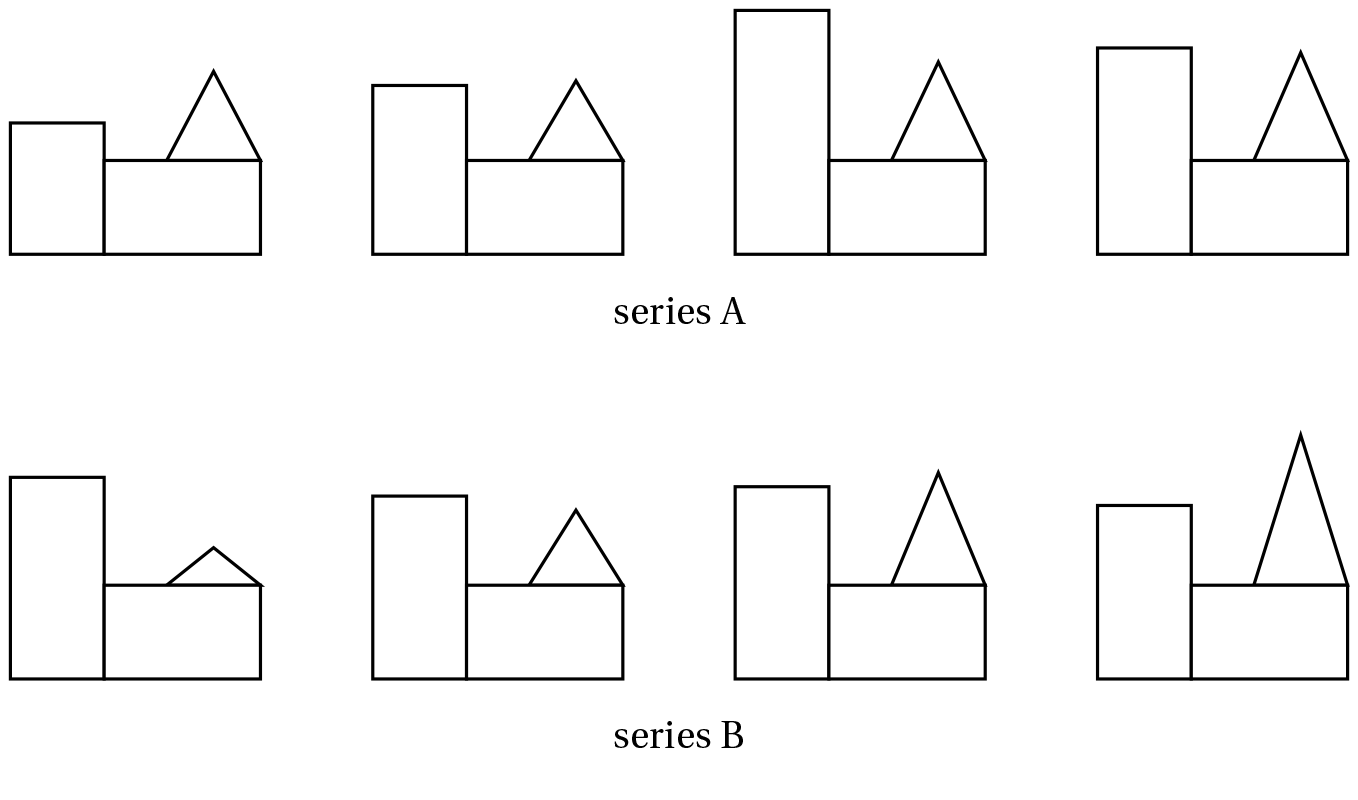
A new set of 24 stimulus designs (see Figure 6.4) was created to meet the goals of the study. These designs were black-and-white abstract line figures constructed out of basic geometric shapes (i.e., rectangles, rectangular triangles, and equilateral triangles). The number of basic shapes from which a design was constructed varied between two and five basic shapes (4 designs with two basic shapes, 8 with three basic shapes, 8 with four basic shapes, and 4 with five basic shapes). Within each design, two feature dimensions were varied. These dimensions were selected to be variable in a quantitative way, because they needed to vary in intensity rather than content (Gati & Tversky, 1982), and to be perceptually separable, because selective attention to separate dimensions was necessary to make independent decisions about a single feature dimension (Dunn, 1983). The possible feature dimensions included: height or width of one of the basic shapes, or the position of a point of a triangle relative to its opposite side. By means of varying these feature dimensions quantitatively, for each design two series of four stimuli were constructed, an A and a B series (see Figure 6.5). In the A series, the variability on the first feature dimension was higher than the variability on the second feature dimension, whereas in the B series the variability on the second feature dimension was higher that the variability on the first feature dimension. Specific rules were followed to determine the range of the feature values and to select the possible target stimuli (see Appendix D).
6.2.3 Procedure
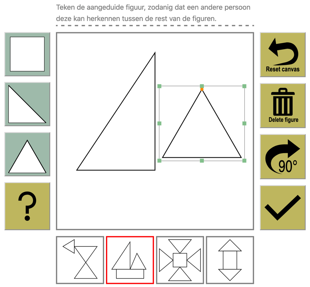
The study was conducted online, and was programmed in HTML, CSS, and JavaScript, using the jsPsych 6.1 and Fabric.js 4.2 JavaScript libraries (de Leeuw, 2015; http://fabricjs.com/). At the start of the experiment, participants were briefly informed about the general procedure, and were asked for informed consent to participate in the experiment. To fix the size of the stimuli in the experiment independent of the screen resolution of the participant, a resizing procedure was introduced, in which the participant resized a rectangular container on the screen to match the size of a particular physical object (i.e., student card, identity card, or bank card). The scaling factor was then applied to the rest of the experiment. Participants were instructed to sit at an arm’s length distance directly in front of the screen, and to keep that distance as constant as possible throughout the experiment. After providing their gender and age, participants were redirected to a practice trial. In the practice trial, participants were given the task instructions and the online interface was explained. Before continuing to the experimental task, participants were able to try out the interface (see Figure 6.6) themselves.
In each trial, participants were presented with a set of four stimuli (100 x 100 user units each), simultaneously shown in boxes at the bottom of the screen. The box around the target figure was outlined in red. The goal of the participant in each trial was to construct the target figure by means of basic geometric shapes, in such a way that someone else would be able to recognize it among the other figures shown next to it.
20 out of 24 designs consisted of one or more additional shapes that did not contain a relevant feature dimension. When the target was of one of those designs, the additional shapes (from now on referred to as background shapes) were already depicted on the canvas, to make the task less demanding and more controlled (line width = 2 user units, 500 x 500 user units). To allow for additional space to sharpen the relevant feature dimension, the ratio of the size of these additional shapes to the size of the stimuli presented was 4:1 (whereas the canvas size was 5:1). The basic shapes (i.e., rectangles, rectangular triangles, and equilateral triangles) were presented as buttons on the left side of the screen. When they were clicked, the requested shapes appeared on the left side of the canvas. Participants were able to reposition and rescale a shape, as well as make it higher, lower, wider and narrower. The position of the top point of the equilateral triangle could be moved horizontally. By means of separate buttons, participants could also rotate the shape in steps of 90 degrees, remove it from the canvas, or clear the canvas entirely. Participants received unlimited time to construct the figures. When participants were unsure about the instructions during the experiment, they could click a help button that made the instructions reappear. When they completed a drawing, participants had to click a button to go to the next trial. It was only possible to proceed when at least two shapes were added to the canvas, otherwise they received the following warning message: “Attention! The drawing is not yet complete”.
Across trials, the similarity of the target to the distractors was manipulated, yielding two types of contexts, the close and the far context (see Figure 6.3). In the close context, target and distractors differed only quantitatively on the two relevant feature dimensions, whilst they were qualitatively the same, making the values on the dimensions potentially important for discrimination. In the far context, target and distractors were qualitatively different, making the values on the dimensions rather unimportant for discrimination.
Independently for each participant, the 24 designs were randomly assigned a context, i.e., close or far, such that 12 designs were presented in a far and 12 designs were presented in a close context. Within each context condition, for six designs series A and for six designs series B was presented. Within each series and context condition, one of the two possible targets was randomly chosen, such that three times the target with the minimum value on the dimension with the largest variability was used, and three times the target with the maximum value on the dimension with the largest variability was used. The trial order as well as the position of target and distractor stimuli in a series was randomized. Participation took approximately 30 minutes. After completion, participants could indicate whether they wanted to receive the debriefing about the main goals and/or the results of the study.
6.2.4 Data analysis
We used R [Version 4.0.4; R Core Team (2021)] for all our analyses.2
6.2.4.1 Preprocessing
Several preprocessing steps were required before we could calculate the relevant measures of interest (see Appendix D). Difference scores were then calculated between the drawn feature values and the target values, with negative values indicating leveling and positive values indicating sharpening.
6.2.4.2 Qualitative analyses
In the qualitative analyses of the data, we used drawn feature values relative to the available drawing space on the canvas (for sharpening and leveling combined) to calculate the proportion of times a feature dimension was leveled or sharpened depending on the context and variability conditions.3 We defined leveling and sharpening in multiple ways. Firstly, we defined leveling as a drawn value on the same side of the target value as the mean, and sharpening as a drawn value equal to the target value or more extreme (i.e., on the other side of the target value compared to the mean). Secondly, we included a third, ‘neutral’ category around the target value which could be seen as equivalent to the target value (only possible when using the relative feature values, i.e., relative to the available space for drawing a specific feature dimension). Thirdly, we explored an alternative definition of leveling as a drawn feature value closer to the mean than to the target, and sharpening as a drawn feature value being closer to the target than to the mean. The results for this last interpretation are available in Appendix D.
To visualize the data, we plotted the proportion of times a feature value was leveled or sharpened, separate for each context and variability condition, with feature dimensions as data points. Using the qualitative data, we were interested in investigating whether the proportion of sharpening was higher (and the proportion of leveling was lower) for (a) drawings in the close context compared to the far context; (b) feature dimensions exhibiting major variability rather than minor variability (especially in the close context); and (c) feature values on an extreme of the dimension rather than exhibiting an in-between value (especially in the close context). To investigate our research questions, we fitted hierarchical regression models using the brms (Bürkner, 2017, 2018) package in R (see below as well as Appendix D for more information).
For each of the definitions of sharpening, we fitted a hierarchical Bayesian binomial regression model to the proportion of times a dimension was sharpened, with context, variability, and their interaction as fixed effects and feature dimension and participant ID as random effects for both intercept and slopes. Given the second definition of sharpening, i.e., including a neutral range around the target value, we also fitted hierarchical Bayesian binomial regression models to the proportion of times a dimensions was leveled or in the 5% range around the target value.
To investigate whether the proportion of sharpening, leveling, or being in target range was higher for drawings in the close compared to the far context, for major compared to minor variability dimensions, and for extreme compared to non-extreme feature values, we plotted the posterior estimates from the model and compared the slope strengths across conditions by plotting contrast distributions for the slopes.
6.2.4.3 Quantitative analyses
In the quantitative analyses, we used the drawn feature values relative to the available drawing space on the canvas. We explored whether the extent to which a feature was leveled or sharpened differed between context and variability conditions. It is important to keep in mind that given the definition of the feature values relative to the total available drawing space (for leveling and sharpening combined), the available range for sharpening was bigger for dimensions with less variability, leading to a conservative estimate for the variability and extremeness effects.
To visualize the data, we plotted the difference between the drawn feature value and the target feature value relative to the available drawing space for that feature dimension, separate for each context and variability condition, with feature dimensions as data points. Using the quantitative data, we were interested in investigating whether the extent to which a feature was sharpened was on average larger for (a) drawings in the close context compared to the far context; (b) feature dimensions exhibiting major variability rather than minor variability (especially in the close context); and (c) feature values on an extreme of the dimension rather than exhibiting an in-between value (especially in the close context). Also for the quantitative data, we fitted hierarchical regression models using the brms (Bürkner, 2017, 2018) package in R to answer our research questions (see below as well as Appendix D for more information).
We fitted a hierarchical Bayesian regression model to the difference in feature value between drawing and target, with context, variability, and their interaction as fixed effects and feature dimension and participant ID as random effects for both intercept and slopes. To investigate whether the extent of sharpening was larger for drawings in the close compared to the far context, for major compared to minor variability dimensions, and for extreme compared to non-extreme feature values, we plotted the posterior estimates from the model and compared the slope strengths across conditions by plotting contrast distributions for the slopes.
6.3 Results
6.3.1 Qualitative analysis
6.3.1.1 Traditional interpretation of leveling and sharpening (binarized; relative values)
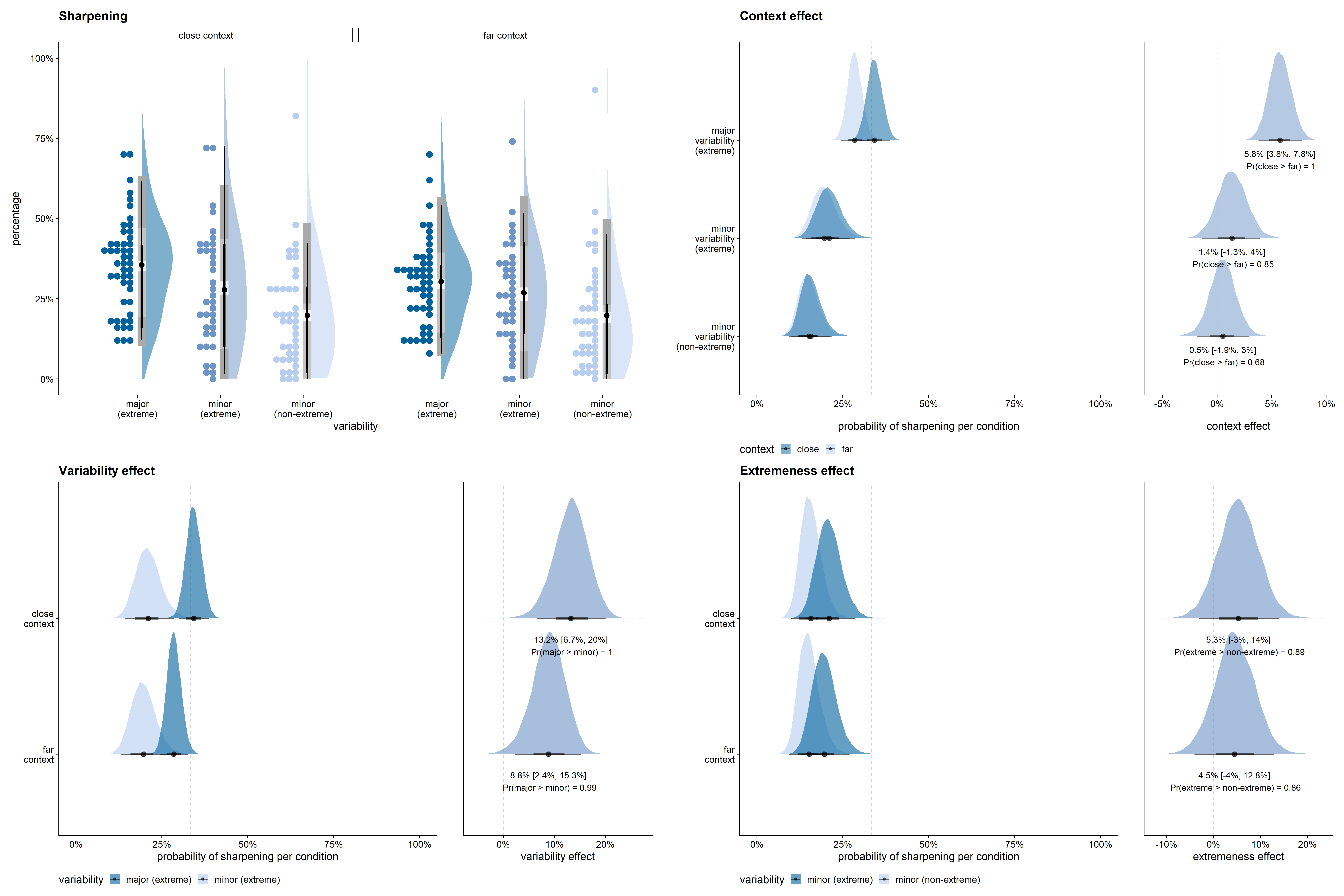
Figure 6.7 shows the empirical percentage of drawings in which each of the 48 feature dimensions was sharpened, separately for each context (i.e., close or far) and variability (i.e., major extreme, minor extreme, minor non-extreme) condition, as well as the distribution across feature dimensions. In this figure, sharpening is defined as a drawn value equal to or more extreme than the target value (i.e., on the other side of the target value compared to the mean). As expected, Figure 6.7 indicates that sharpening was more likely for the major variability dimension than for the minor variability dimensions, and that sharpening was more common in the close than in the far context. Furthermore, it is clear that there was much more variability in the percentage of sharpening across feature dimensions in the minor variability conditions than in the major variability condition.
To investigate the effects of context, variability, and extremeness in more detail, we plotted the posterior estimates from the model and compared the slope strengths across conditions by plotting contrast distributions for the slopes.
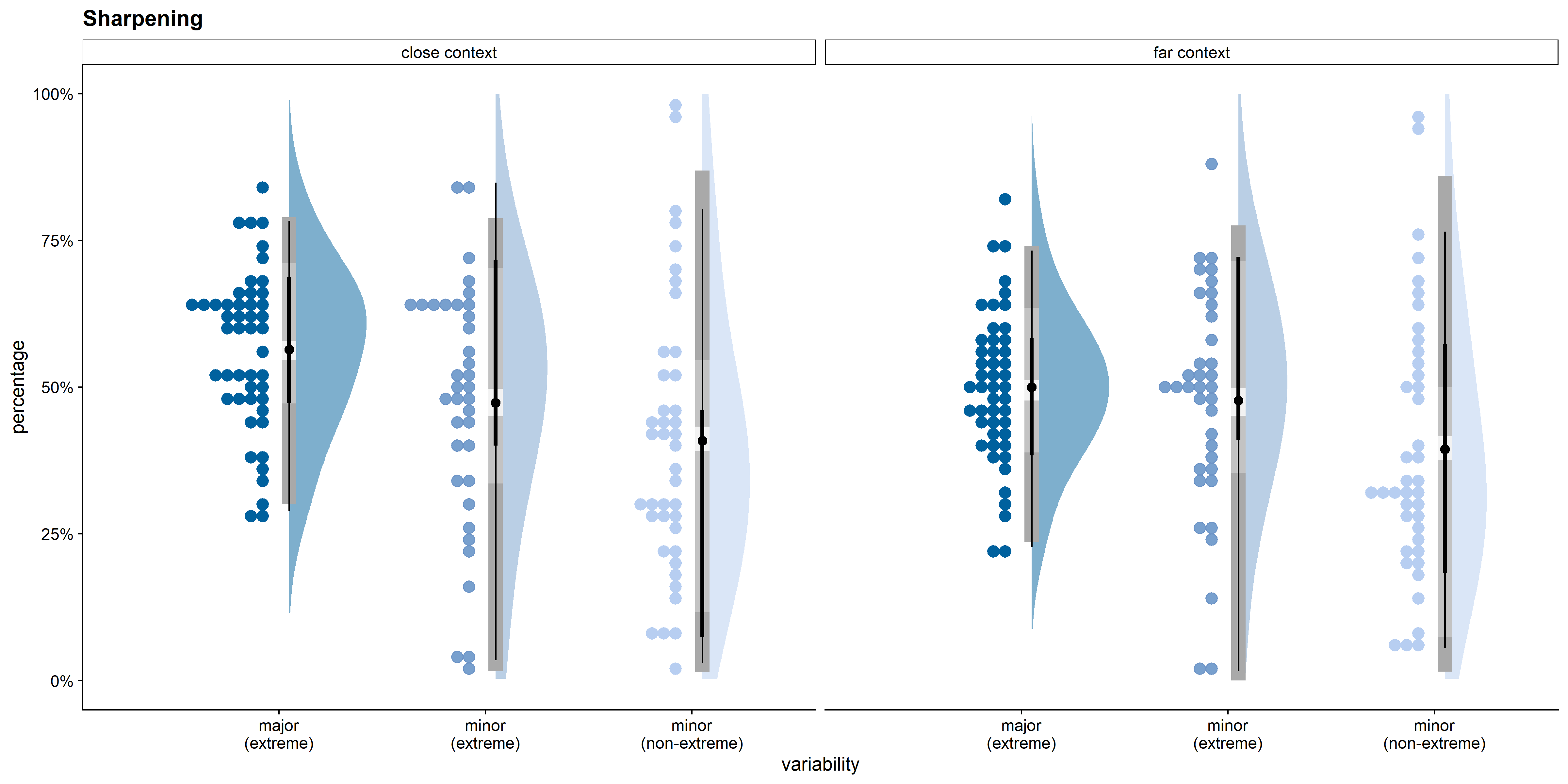
Figure 6.8 visualizes the estimated context effect per variability condition. Especially in the major variability condition, there was a clear effect of context on the probability that the feature was sharpened: in all posterior samples, the probability for the major feature dimension to be sharpened was higher in the close than in the far context. Given that the model is a good approximation of the data, the data provide evidence for a clear context effect in the major variability condition. For the minor variability conditions, the context effect was less clear.
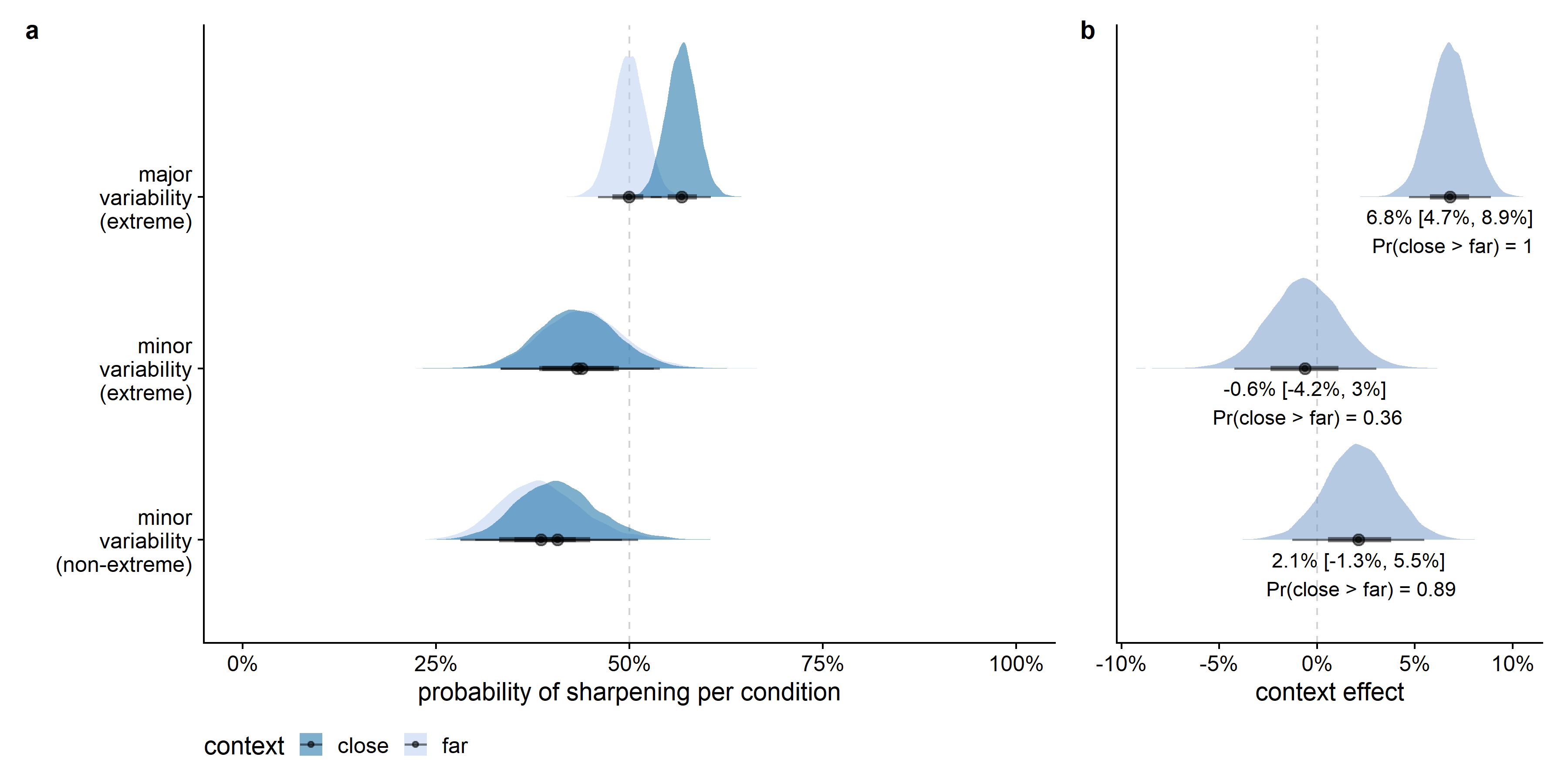
Figure 6.9 pictures the estimated variability effect per context condition. Within the close context, there was a clear effect of the range of variability present on a dimension on the probability that the feature was sharpened: in all posterior samples, the probability for an extreme value on the major feature dimension to be sharpened was higher than the probability for an extreme value on a minor feature dimension. Given that the model is a good approximation of the data, the data provide evidence for a clear effect of variability in the close context condition. In the far context condition, the posterior probability of the proportion of sharpening for an extreme value on a major feature dimension to be larger than for an extreme value on a minor feature dimension was 89%.
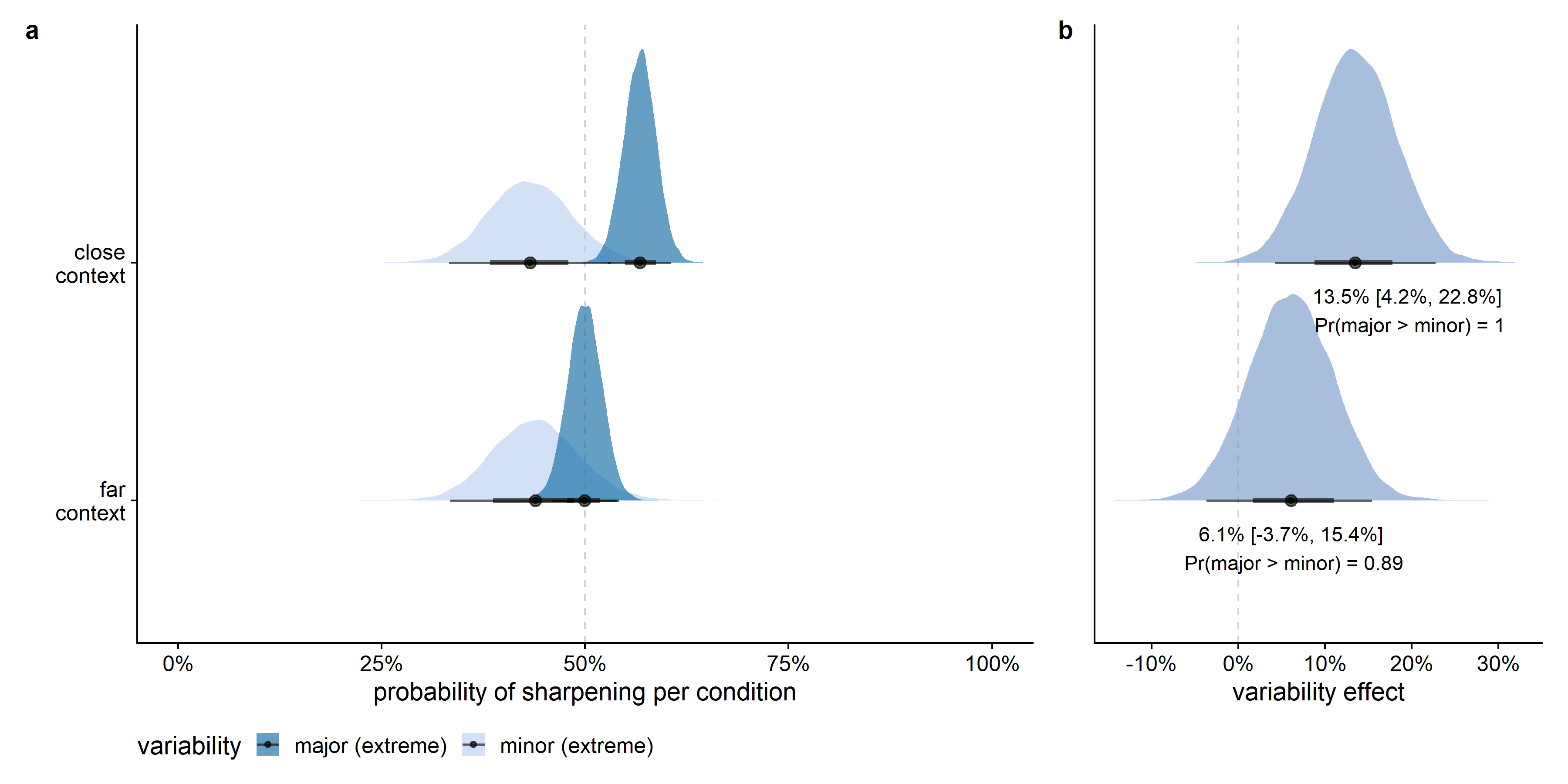
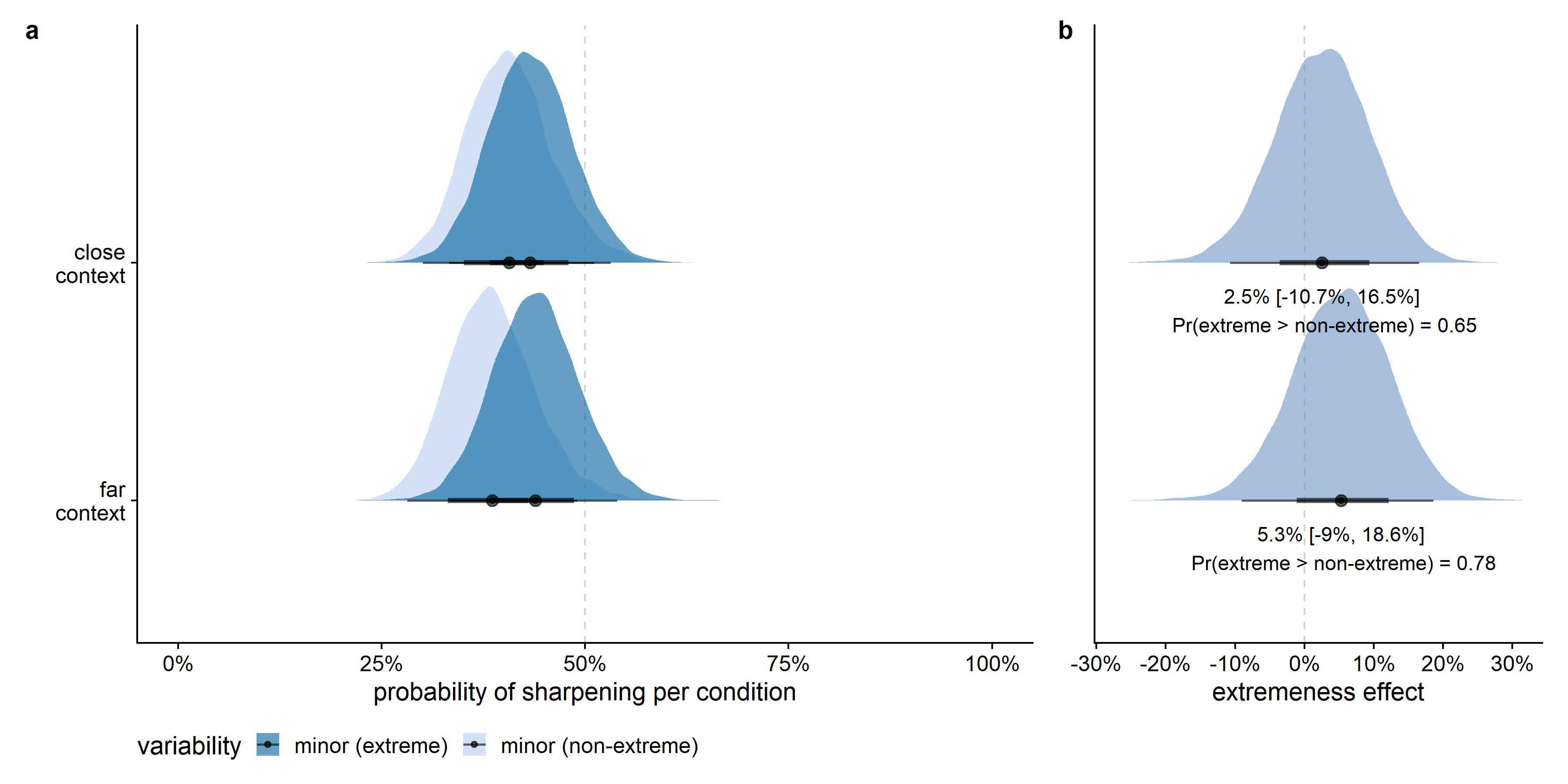
Figure 6.10 shows the estimated extremeness effect per context condition. Within both the close and the far context, there was a tendency for extrema on a feature dimension to be sharpened more often than non-extreme values on feature dimensions with an equal variability range, but in both conditions the 95% HDCI for the difference between an extreme and a non-extreme feature value on the minor dimension included zero as well as differences in the opposite direction.
Additional results concerning the random effects per feature dimension and individual are provided in Appendix D.
Independent of the fitted model, we plotted the empirical percentage of drawings in which each of the 48 feature dimensions was sharpened, separately for each context (i.e., close or far), variability (i.e., major extreme, minor extreme, minor non-extreme), and target (maximum/above mean, minimum/below mean) condition, as well as the distribution across feature dimensions. From visual exploration of the figure, there seems to be no overall effect of target condition on the proportion of times a feature was sharpened (see Figure 6.11).
6.3.1.2 Traditional interpretation of leveling and sharpening including neutral category (relative values)
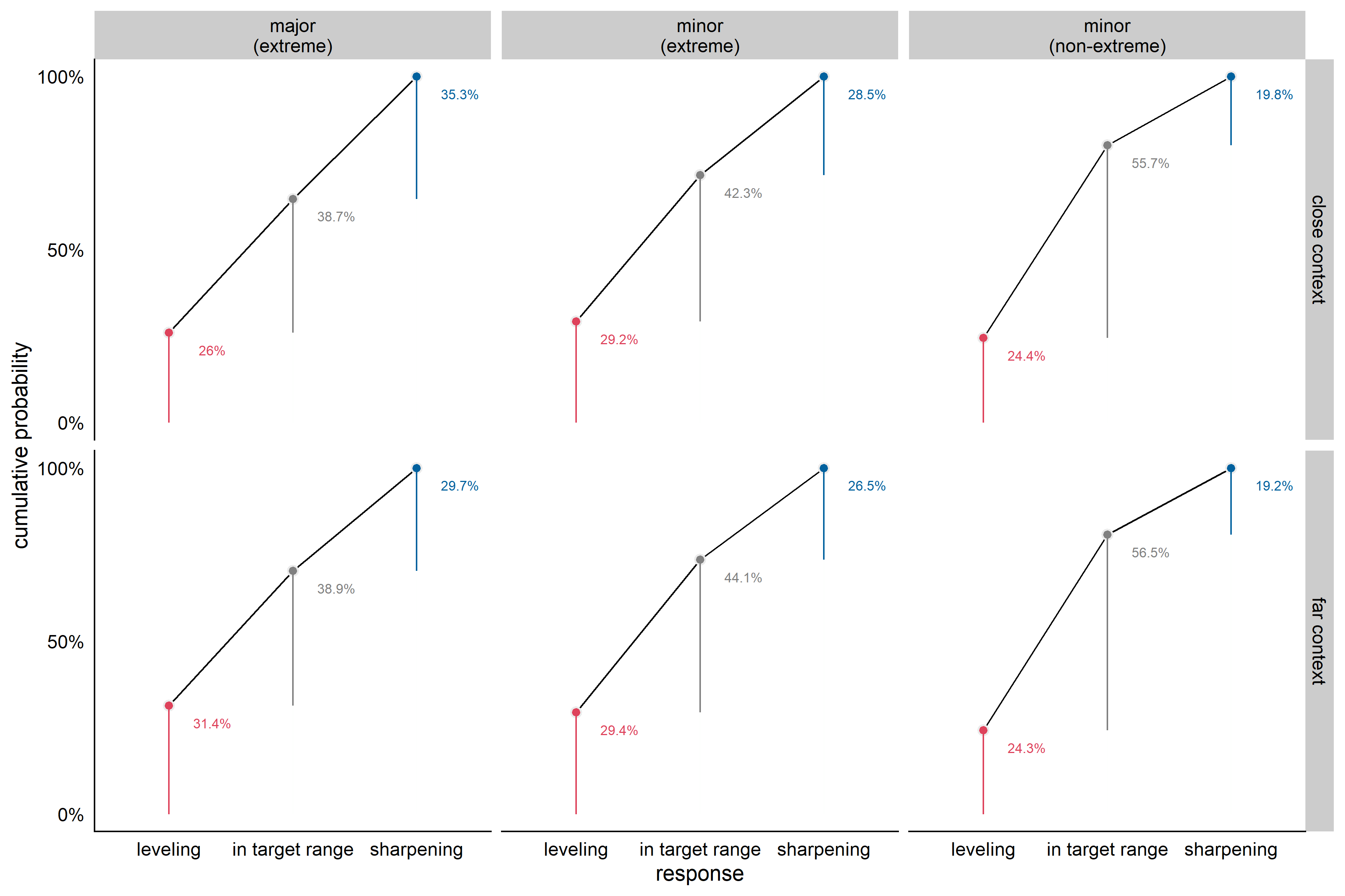
Figure 6.12 shows the empirical percentage of drawings in which a feature dimension was leveled, in a 5% range around the target, or sharpened, averaged across all feature dimensions and participants. From this figure, it is clear that the number of drawn values in the target range increased for the minor non-extreme variability condition compared to the minor extreme variability condition (i.e., extremeness effect), and for the minor extreme variability condition compared to the major extreme variability condition (i.e., variability effect). The opposite trend was observed for the number of sharpened feature values: sharpening was more prominent in the major extreme condition than in the minor extreme condition (i.e., variability effect) and in the minor extreme condition than in the minor non-extreme condition (i.e., extremeness effect). In addition, the number of sharpened drawings seems to be larger in the close than in the far context, especially for the major variability dimension (i.e., context effect). Furthermore, the number of leveled feature values seems to be higher for the extreme variability conditions than for the non-extreme variability condition (i.e., extremeness effect).
The top left graph in Figure 6.13 shows the empirical percentage of drawings in which each of the 48 feature dimensions was sharpened, separately for each context (i.e., close or far) and variability (i.e., major extreme, minor extreme, minor non-extreme) condition. In this figure, sharpening is defined as a drawn value 2.5% away from the target value and more extreme than the target value (i.e., on the other side of the target value compared to the mean). As for the binary definition of sharpening, the figure indicates that sharpening was more likely for the major variability dimension than for the minor variability dimensions, and that sharpening was more common in the close than in the far context. Moreover, there was slightly more variability in the percentage of sharpening across feature dimensions in the minor variability conditions than in the major variability condition.
To investigate the effects of context, variability, and extremeness on the probability of sharpening a feature in more detail, we plotted the posterior estimates from the model and compared the slope strengths across conditions by plotting contrast distributions for the slopes.
The top right graph in Figure 6.13 visualizes the estimated context effect per variability condition. Concerning the major feature dimension, there was a clear effect of context on the probability that the feature was sharpened: in all posterior samples, the probability of sharpening was higher in the close context than in the far context condition. Within both the close and the far context, there was a clear effect of the range of variability present on a dimension on the probability that the feature was sharpened (see bottom left graph in Figure 6.13): in 100% and 99% of the posterior samples respectively, the probability for an extreme value on the major feature dimension to be sharpened was higher than the probability for an extreme value on a minor feature dimension to be sharpened. Within both the close and the far context, there was a slight tendency for extrema on a feature dimension to be sharpened more often than non-extreme values, on feature dimensions with an equal variability range. In the close and far context conditions, the posterior probability of the proportion of sharpening for an extreme value on a minor feature dimension to be larger than for a non-extreme value on a minor feature dimension were 89% and 86%, respectively.
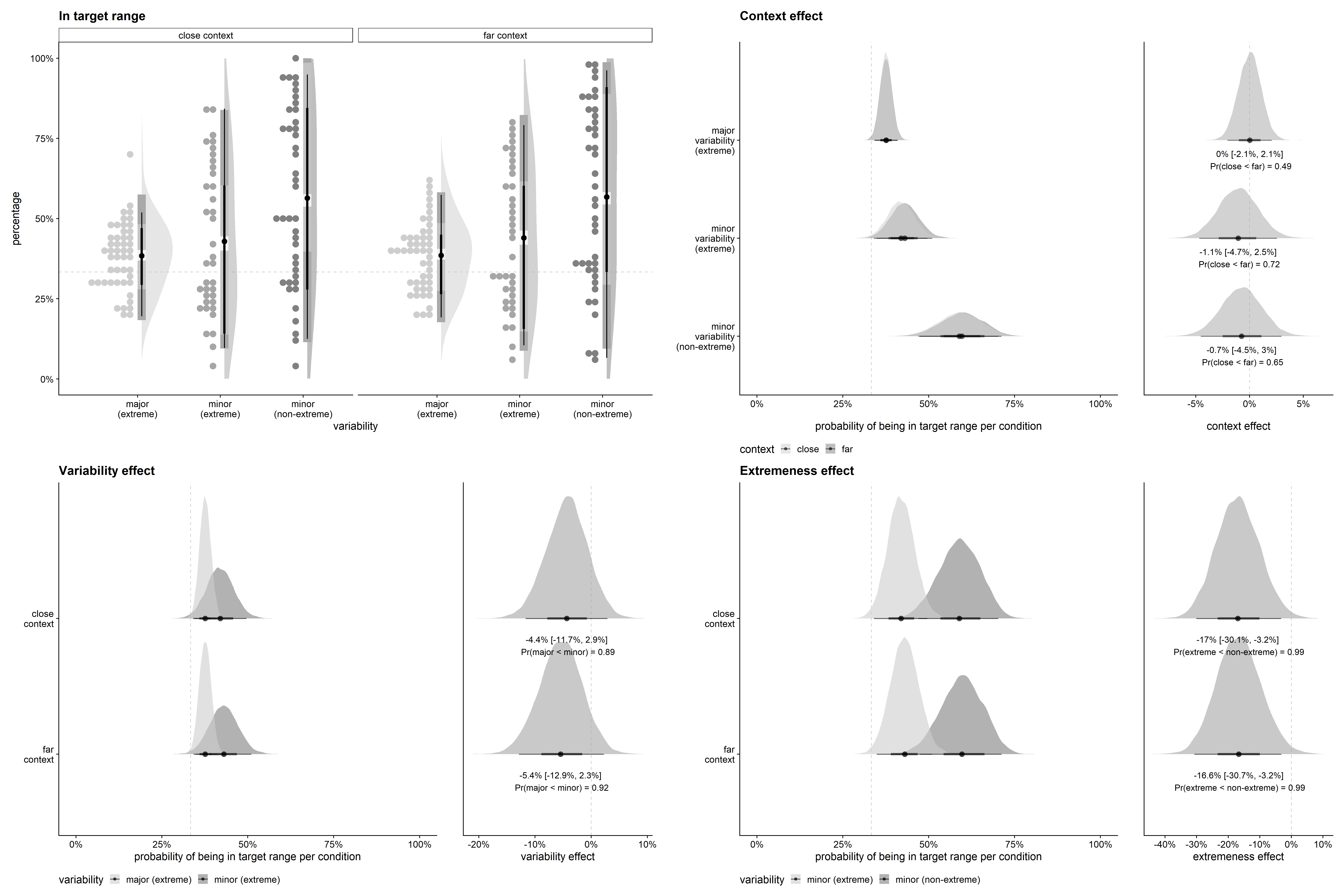
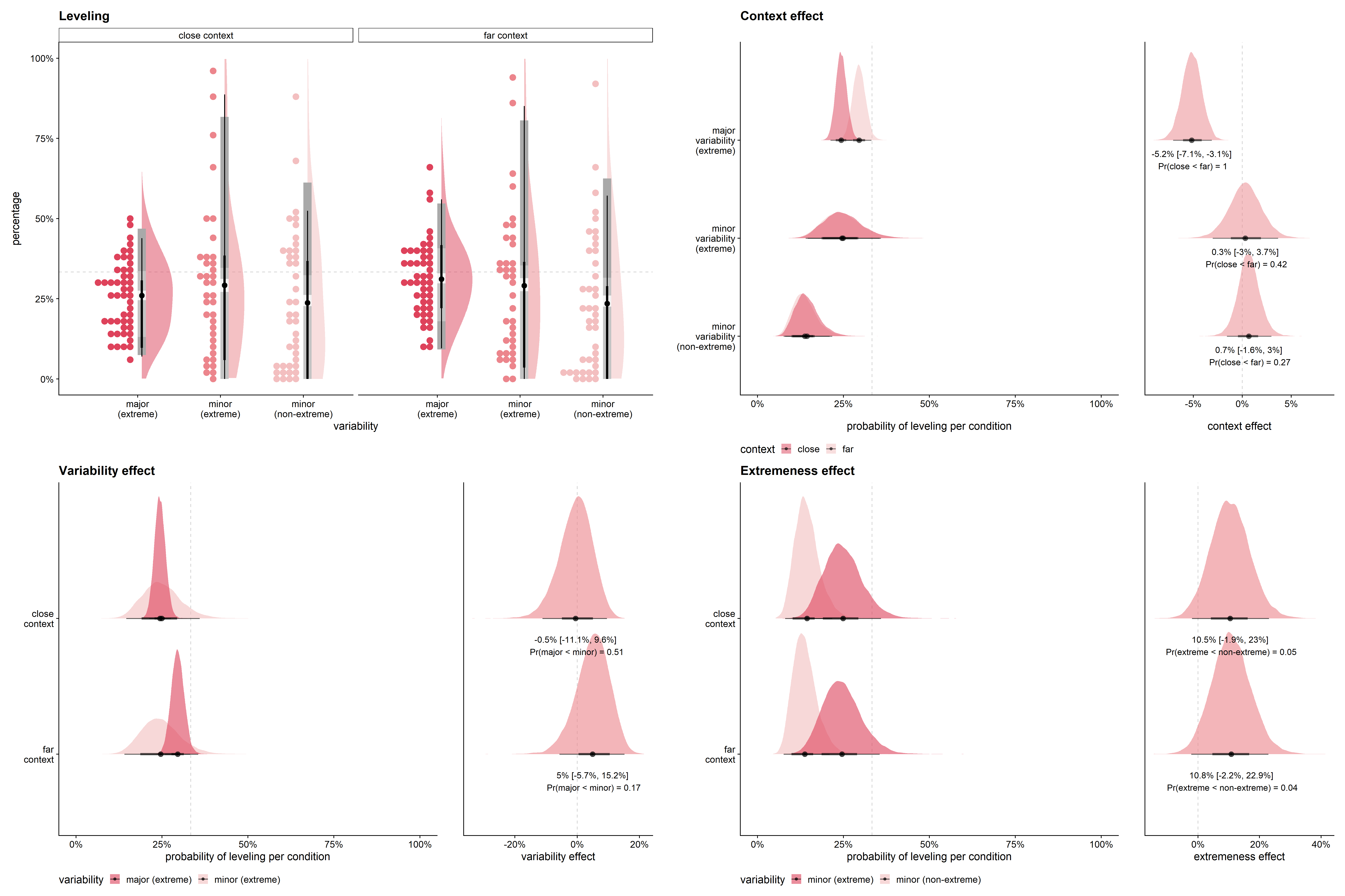
Figure 6.15 visualizes the estimated effects of context, variability, and extremeness for the probability of leveling a feature value. Concerning the major feature dimension, there was a clear effect of context on the probability that the feature was leveled: in all posterior samples, the probability of leveling was higher in the far context than in the close context condition. No clear effect of the range of variability present was found on the probability that a feature was leveled (see bottom left graph in Figure 6.15). Within both the close and the far context, there was a tendency for extrema on a feature dimension to be leveled more often than non-extreme values on feature dimensions with an equal variability range. In the close and far context conditions, the posterior probability of the proportion of leveling for an extreme value on a minor feature dimension to be larger than for a non-extreme value on a minor feature dimension were 95% and 96%, respectively.
Figure 6.14 visualizes the estimated effects of context, variability, and extremeness for the probability of drawing a feature within the target range. There was no clear effect of context on the probability that the feature was in the target range. Within both the close and the far context, there was a tendency for the minor variability dimension to be in target range more often than the major variability dimension (see bottom left graph in Figure 6.14). Within both the close and the far context, there was a clear effect of extremeness: non-extreme feature values on a feature dimension were more often in target range than extreme values, on feature dimensions with an equal variability range. In both the close and the far context condition, the posterior probability of the proportion of being in target range for a non-extreme value on a minor feature dimension to be larger than for an extreme value on a minor feature dimension was 99%.
6.3.2 Quantitative analysis
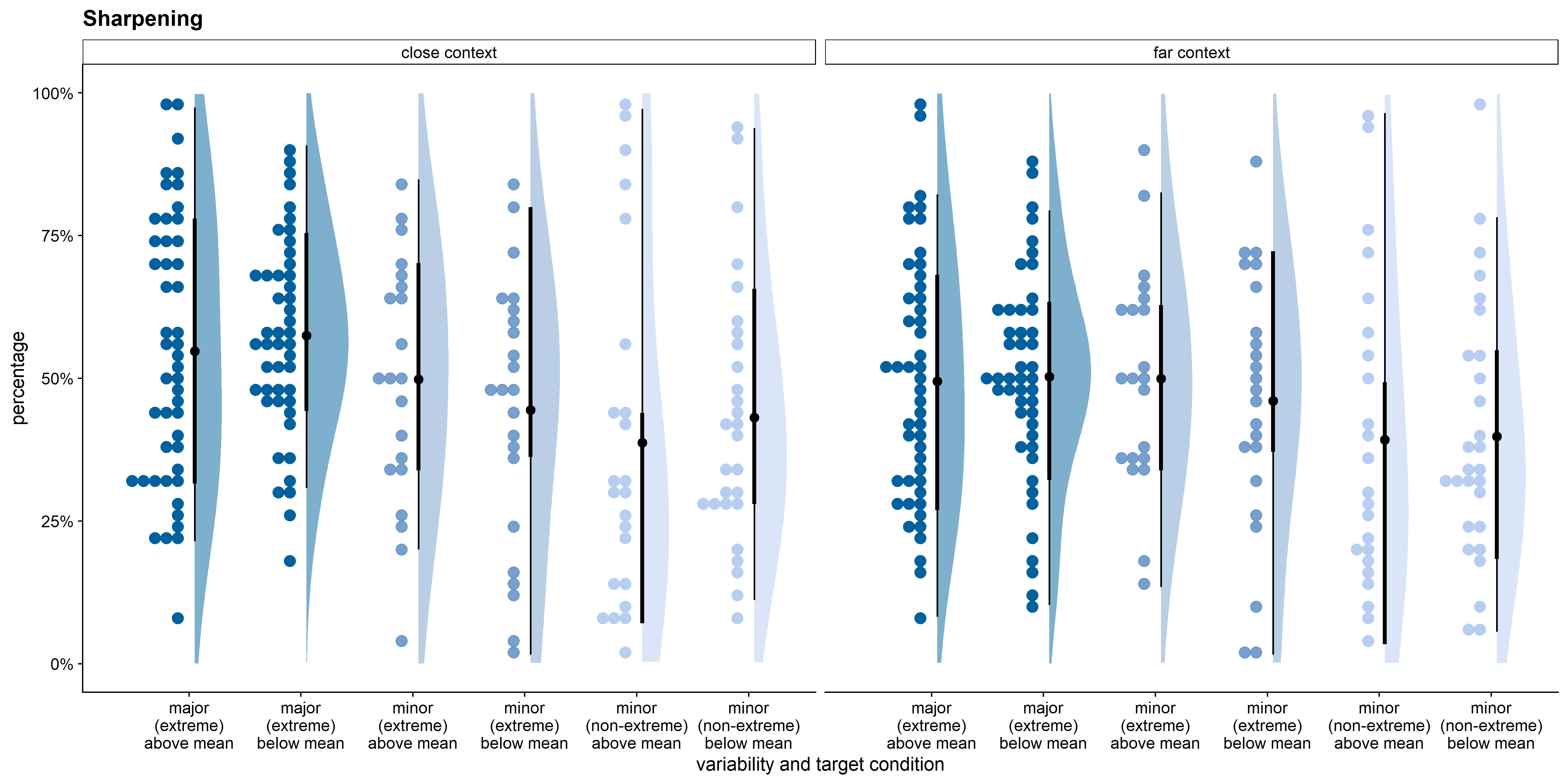
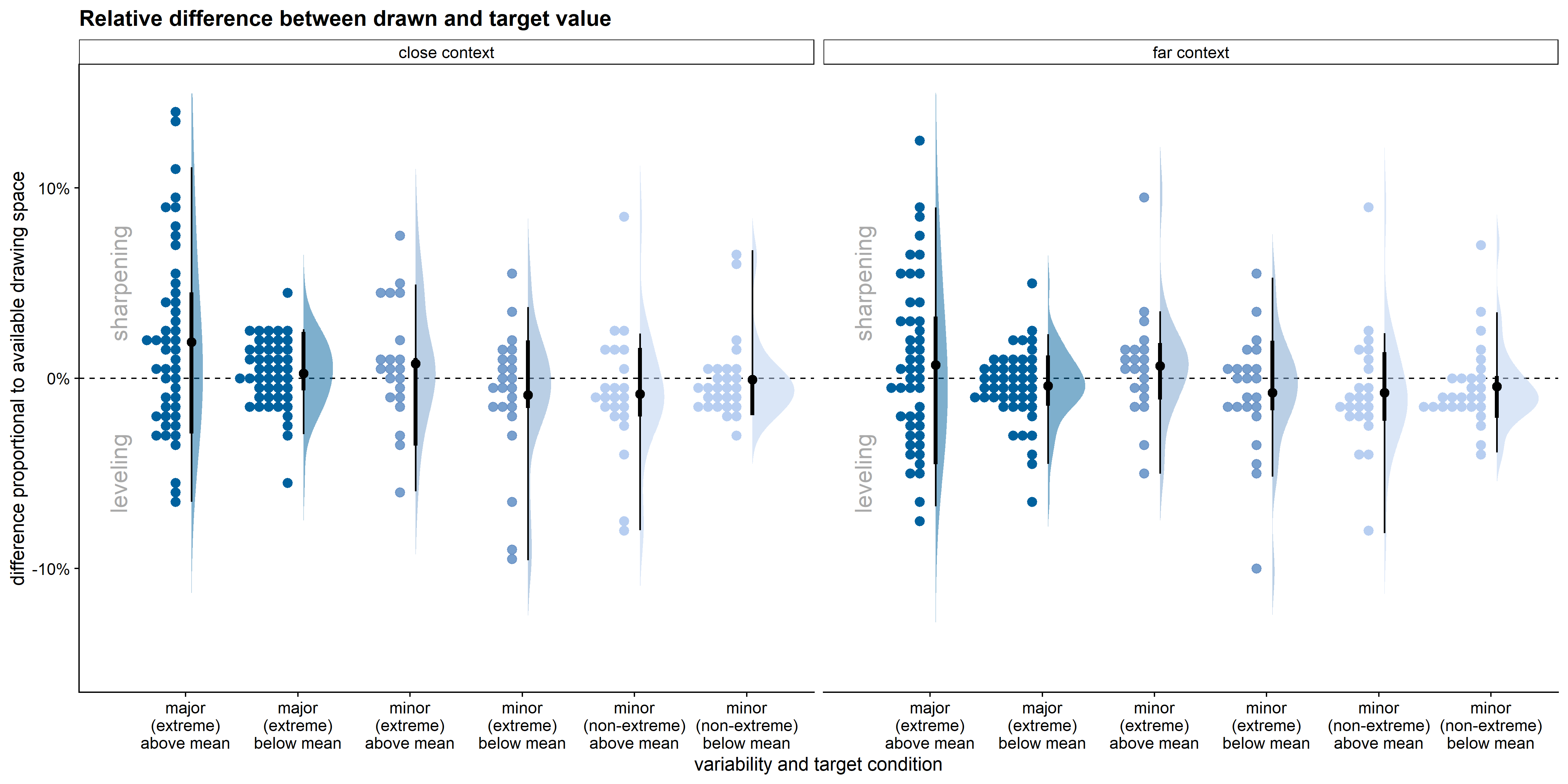
Figure 6.16 shows the distribution of difference between drawn and target value (relative to the available drawing space for that feature dimension), per context and variability condition, with values for individual trials as data points. Figure 6.17 shows the mean empirical difference between drawn and target feature values relative to the available drawing space for each of the 48 feature dimensions, separately for each context (i.e., close or far) and variability condition (i.e., major extreme, minor extreme, minor non-extreme), as well as the distribution across feature dimensions. The figure indicates that the extent of sharpening was on average slightly larger for the major variability dimension than for the minor variability dimensions, especially in the close context.
To investigate the effects of context, variability, and extremeness in more detail, we plotted the posterior estimates from the model and compared the slope strengths across conditions by plotting contrast distributions for the slopes.
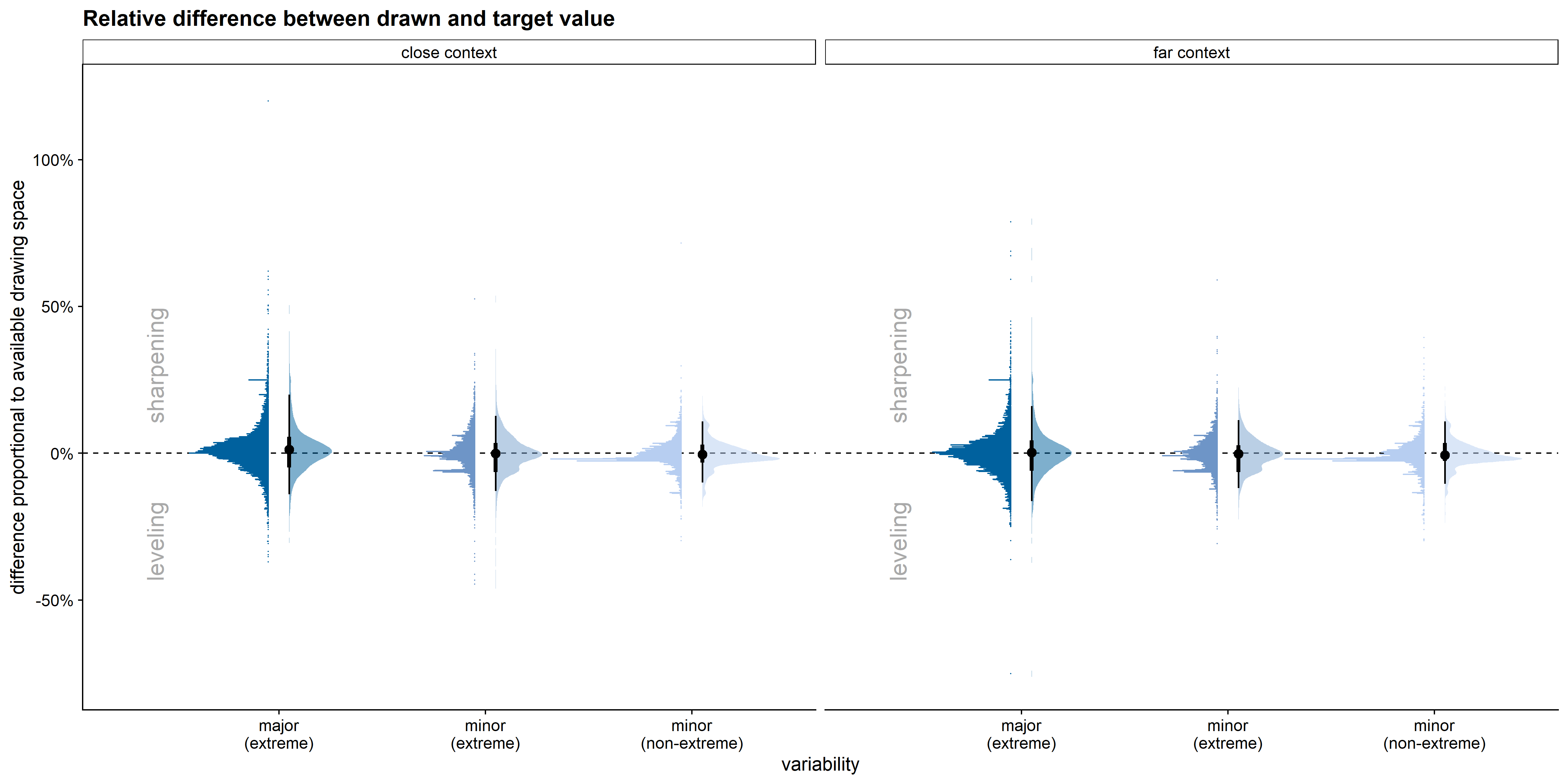
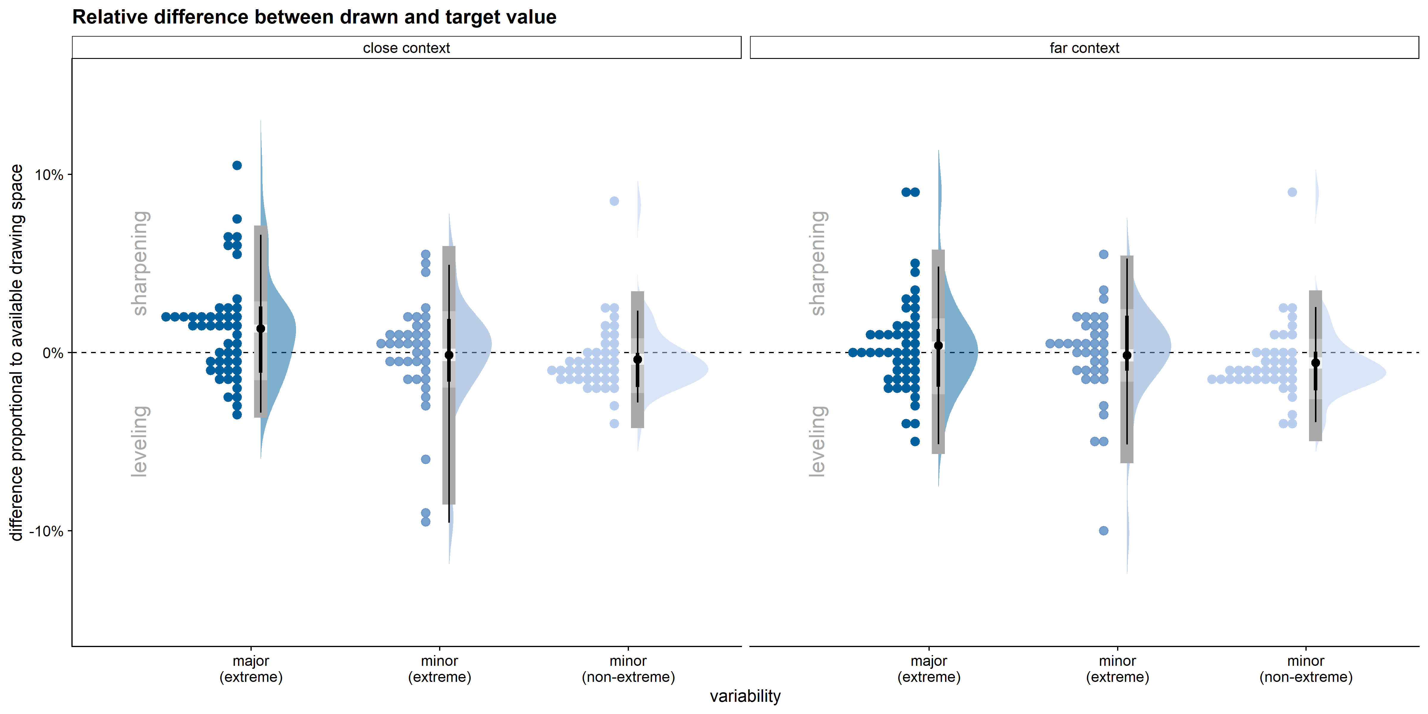
Figure 6.18 visualizes the estimated context effect per variability condition. In the major variability condition, there was a clear effect of context on the extent to which the feature was sharpened: in 99% of the posterior samples, the expected sharpening for the major feature dimension was larger in the close than in the far context. Given that the model is a good approximation of the data, the data provide evidence for a clear effect of context in the major variability condition. For the minor variability conditions, there was no clear effect of context.
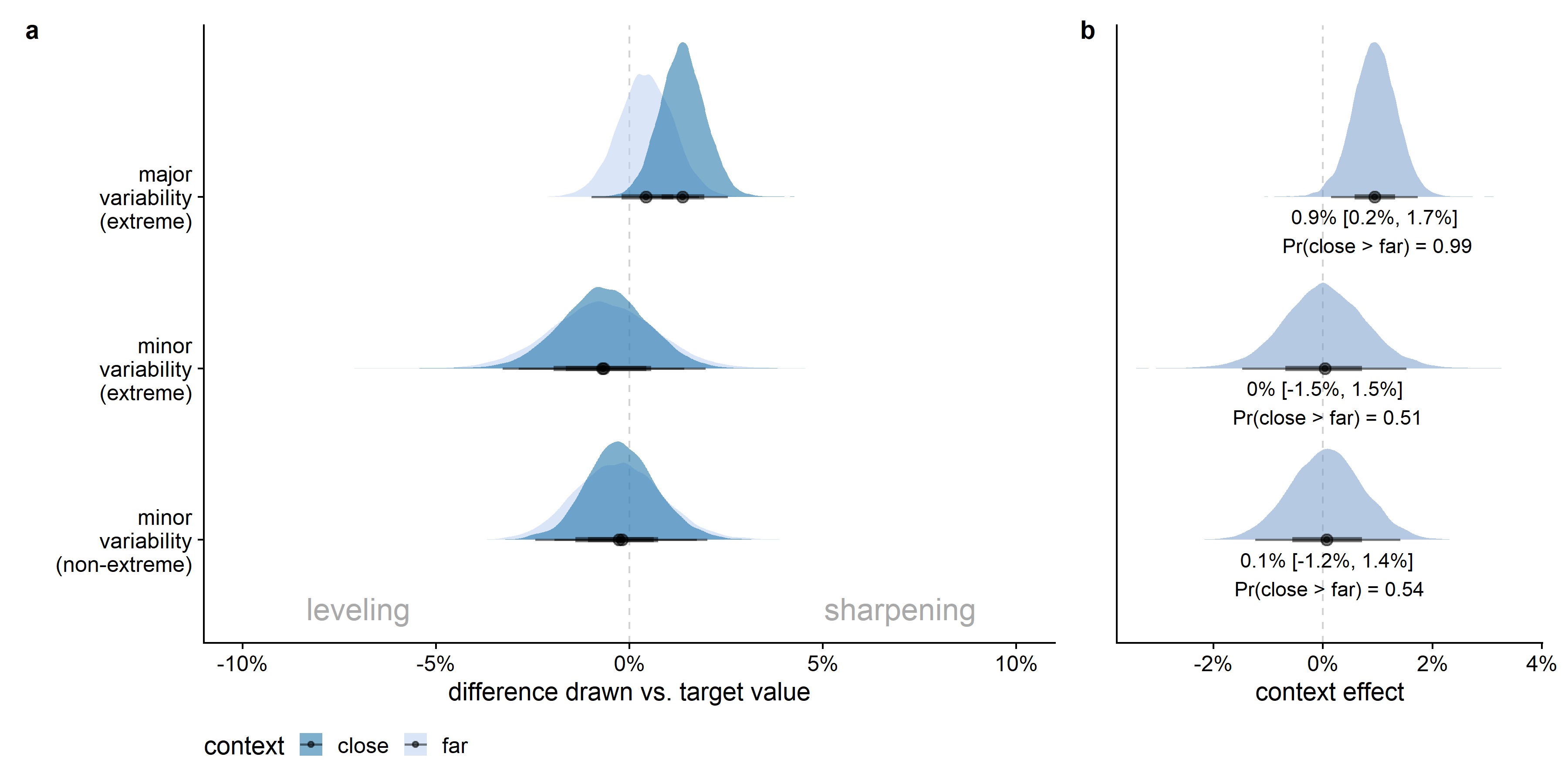
Figure 6.19 pictures the estimated variability effect per context condition. Within the close context, there was a clear effect of the range of variability present on a dimension on the extent to which the feature was sharpened: in 98% of the posterior samples, the expected sharpening for an extreme value on the major feature dimension was higher than for an extreme value on a minor feature dimension. For the far context condition, the variability effect was in the expected direction in 84% of the posterior samples.
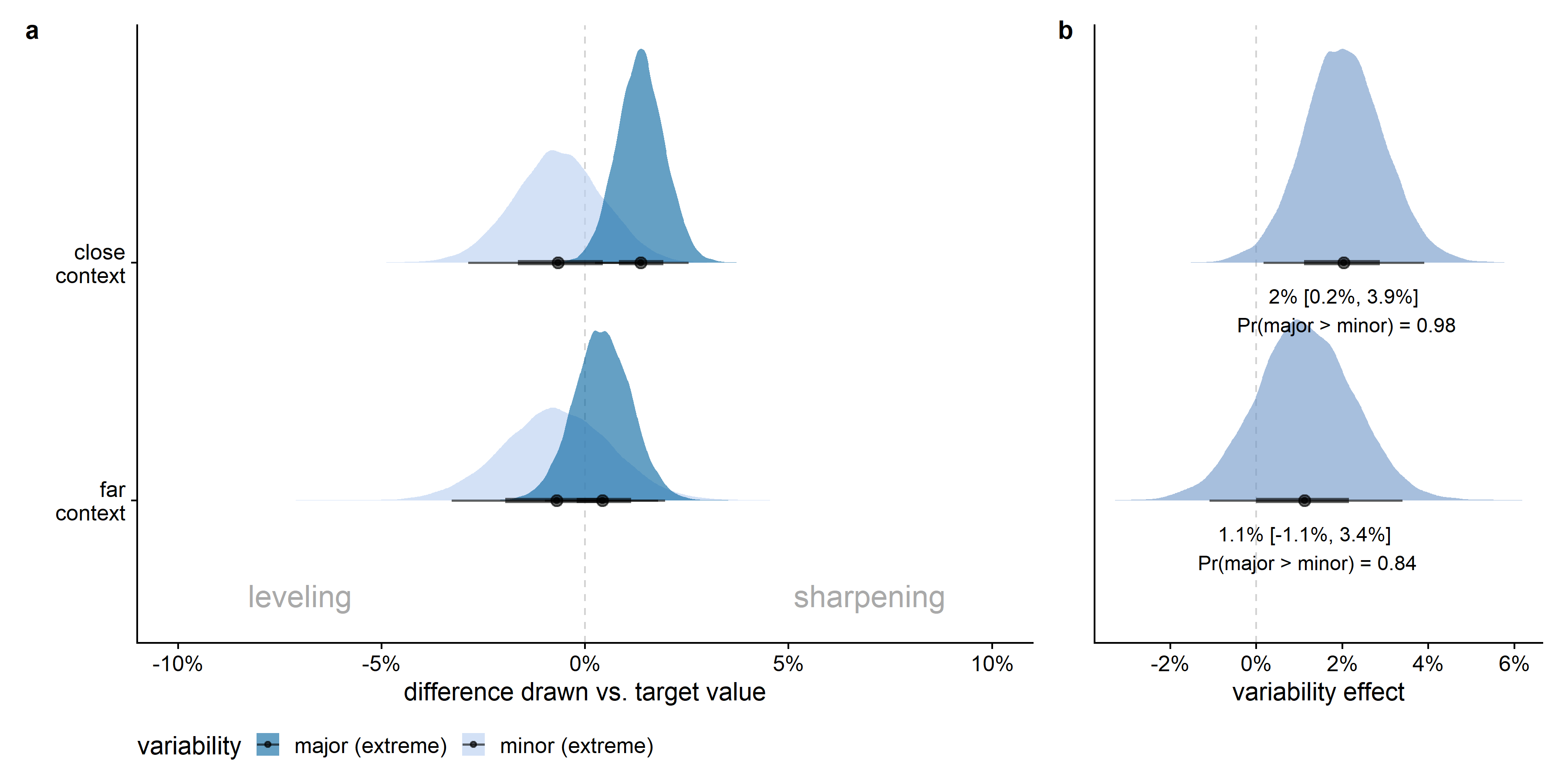
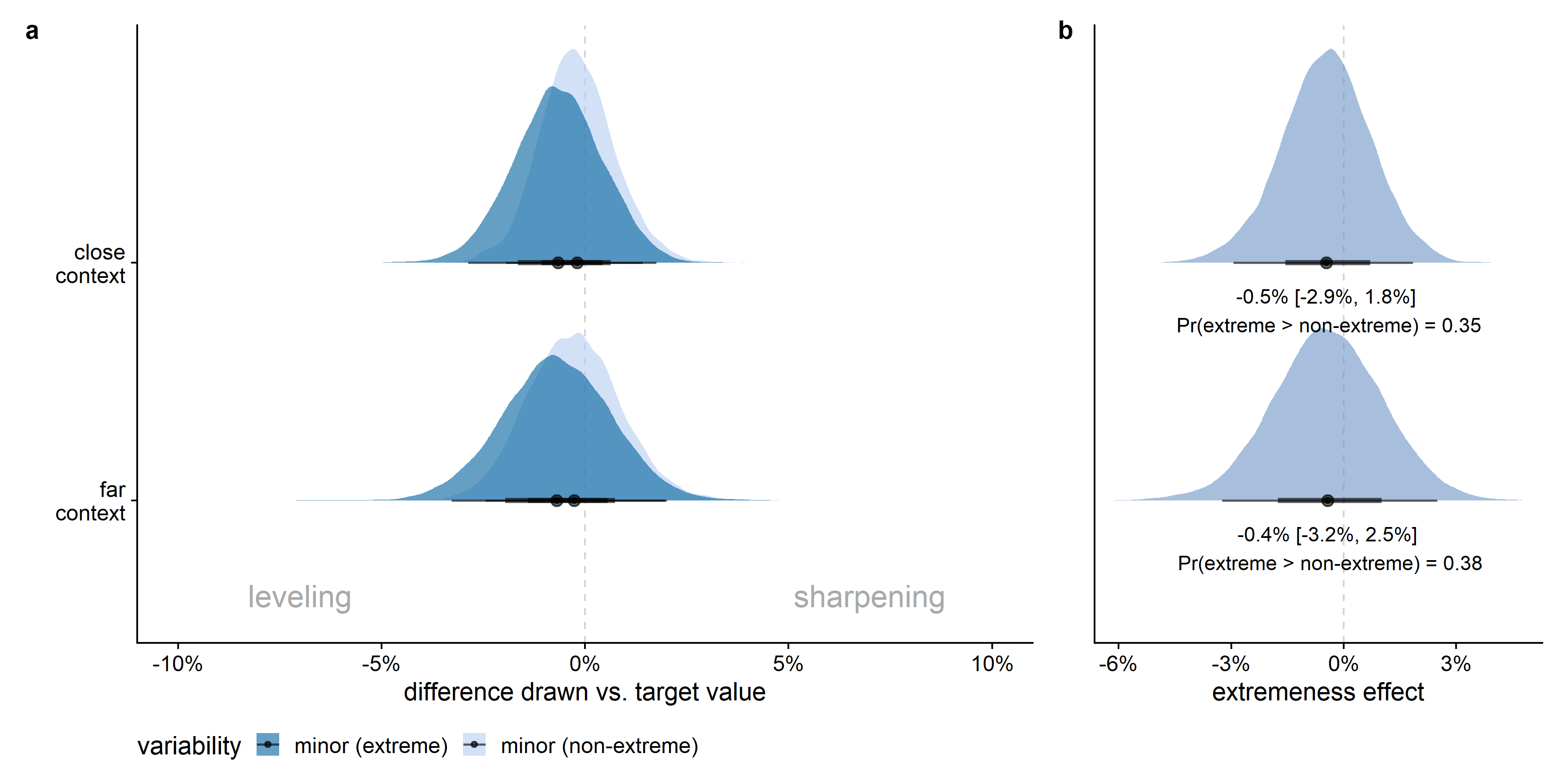
Figure 6.20 shows the estimated extremeness effect per context condition. Within both the close and the far context, there was no evidence for extrema on a feature dimension to be sharpened more often than non-extreme values, on feature dimensions with an equal variability range.
Additional results concerning the random effects per feature dimension and individual are provided in Appendix D.
Independent of the fitted model, we plotted the mean empirical difference difference between drawn and target feature values relative to the available drawing space for each of the 48 feature dimensions, separately for each context (i.e., close or far), variability (i.e., major extreme, minor extreme, minor non-extreme), and target (maximum/above mean, minimum/below mean) condition, as well as the distribution across feature dimensions. From visual exploration of the figure, there seems to be an effect of target condition on the extent to which a feature was sharpened in the major extreme and minor extreme variability conditions (see Figure 6.21). More specifically, the extent of sharpening seems larger in the maximum target conditions (i.e., major extreme above mean and minor extreme above mean) than in the minimum target conditions (i.e., major extreme below mean and minor extreme below mean).
6.4 Discussion and conclusion
6.4.0.1 Summary of the experiment and main results
In this study, we investigated whether the importance of a feature for discrimination within a specific (task) context influences which Prägnanz tendency (i.e., leveling or sharpening) will occur. More specifically, we hypothesized that when a feature is important for discrimination of a target figure from alternative figures, the feature will more often be sharpened (and less often be leveled) than features less important for discrimination within the given context.
Building on the methodology of Fan et al. (2020), we presented participants with four figures consisting of basic geometric shapes and asked them to reconstruct one of these. The figures either differed qualitatively from each other (i.e., far context condition), or only quantitatively on two feature dimensions (i.e., close context condition). Assuming that the quantitative feature differences would play a bigger role in discrimination from the other figures in the close context condition, we expected more sharpening in the close compared to the far context condition, and more leveling of features in the far compared to the close context condition.
Of the two feature dimensions showing variability across the four simultaneously presented figures, one feature dimension showed larger differences than the other feature dimension (i.e., major vs. minor variability). More specifically, the range of feature values was four times wider for the major variability compared to the minor variability condition. Assuming that the major feature dimensions would be more important for discrimination of the target from the alternatives than the minor feature dimension, we expected more sharpening for the major compared to the minor feature dimension, and more leveling for the minor compared to the major feature dimension.
Although the target figure was always either the figure with a minimum or a maximum value on the major feature dimension, target figures varied in whether the value on the minor feature dimension was an extreme value as well or rather an in-between value. Assuming that having an extreme value on a feature dimension is more useful for discrimination from the alternatives than having an in-between value, it could be expected that extreme values would be sharpened more than non-extreme values, and that more leveling would occur for non-extreme than for extreme feature values.
After extensive preprocessing of the data, we investigated both the percentage of times a feature dimension was leveled or sharpened (i.e., qualitative analysis) and the extent to which a feature dimension was leveled or sharpened (i.e., quantitative analysis) using Bayesian hierarchical regression models with context, variability, and their interaction as fixed effects and as random effects per feature dimension and participant.
For the qualitative analysis, we compared different definitions of sharpening and leveling and how they impacted the results. In case sharpening was defined as a drawn value equal or more extreme than the target value (i.e., on the other side of the target value compared to the mean), results indicated a strong effect of context on the percentage of times a feature was sharpened, at least in the major variability condition: sharpening was more likely for major feature values in the close than in the far context. Similarly, in the close context, the major feature dimension was sharpened more often than the minor variability dimension.
When including a neutral category and thus limiting sharpening to drawn values at least 2.5% more extreme than the target value, again a strong effect of context for the major variability condition was found: sharpening was more likely for major feature values in the close than in the far context. Using this definition including a neutral range, the probability of sharpening was influenced by the range of variability present on the dimension in both the close and the far context: sharpening was more likely for dimensions showing major variability than for dimensions showing only minor variability, both in the close and in the far context condition. Furthermore, we found more leveling in the far than in the close context, at least in the major variability condition, but also more leveling for extreme rather than non-extreme feature values. The number of drawings within the target range was higher for non-extreme feature values than for extreme ones.
When defining sharpening as a drawn value closer to the target value than to the mean value on the dimension (see Appendix D), the effect of context diminished, and the effect of variability and extremeness on the percentage of times a feature is sharpened increased. In other words, the drawn value will much more often be closer to the target than to the mean in case it concerns a major variability dimension (compared to a minor variability dimension). In addition, an extreme value on a minor variability dimension will more often be closer to the target than to the mean compared to a non-extreme value on a minor variability dimension.
For the quantitative analysis we compared the difference between drawn value and target value proportional to the available drawing space (for leveling and sharpening combined). The Bayesian hierarchical linear regression model led to similar conclusions as the qualitative analysis: the extent to which a feature was sharpened in the major variability condition was higher in the close compared to the far context condition. In addition, in the close context, the major variability dimension was sharpened more strongly than the minor variability dimension. It is important to take into account that the estimated size of the variability effect is a conservative estimate, given that the measure does not take into account that there is more drawing space available for a minor variability feature to be sharpened than for a major variability feature. Visual inspection of the quantitative data grouped by context, variability, and target condition (i.e., target above or below the mean) hinted at an additional effect of the target type (minimum/below mean vs. maximum/above mean) on the extent to which a feature was sharpened, at least in the major extreme and minor extreme conditions. More specifically, the extent to which a feature was sharpened seemed to be larger in the maximum target conditions than in the minimum target conditions. In the qualitative analysis, no such effect of target type seemed to be present.
In general, we found more evidence for variability between feature dimensions than between participants (see Appendix D), but this result can very likely be attributed to the limited number of data points available per participant (2-48 data points per participant) compared to the number of data points available per feature dimension (400-541 data points per feature dimension). When using the traditional definition of sharpening, we found more uncertainty for the estimates for the effect of context per feature dimension than for the estimated differences between the variability conditions per feature dimension, which is also potentially due to a difference in the number of data points involved in the comparisons.
As repeating the analyses with different data exclusion criteria, and where possible, with absolute scores rather than scores relative to the available drawing space, resulted in similar conclusions and effect sizes as presented in the main text (see Appendix D), the given conclusions are consistent and seem to be robust against such arbitrary choices. Using different definitions of leveling and sharpening led to effects in the same direction, but not always of the same size. Where differences in effect size occurred, presenting the different results gives a more nuanced view on how the results can be interpreted depending on the definitions used.
6.4.0.2 Main conclusions
6.4.0.2.1 Features important for discrimination will more often be sharpened
When a target figure is compared to other figures that only differ from the target figure in a quantitative way, the main distinctive feature will more often be sharpened (i.e., drawn as more extreme than the target value) than when the target is compared to qualitatively different figures (i.e., context effect), especially when it concerns a feature dimension with high variability. Moreover, the main distinctive feature will more often be sharpened than the feature showing only minor variability across figures (i.e., variability effect), especially when figures differ only quantitatively from each other. Similarly, the extent of sharpening is larger in the close compared to the far condition (given a feature showing major variability) and for the major compared to the minor variability dimension (given a close context condition). From these results, we can conclude that a feature will be sharpened more often when this feature is important for discrimination of the target figure from alternatives, compared to when it concerns a feature less important for discrimination. In other words, whether a feature of a figure is important for discrimination, and thus what comprises the essence of the figure, will depend on the context (i.e., the other figures present) in which this figure is presented. As a consequence, the context will also influence which Prägnanz tendency will occur for a specific feature (i.e., leveling or sharpening). The results of this study are in line with recent work by Feldman (2021), who concluded that the improvement in perceptual discrimination of a feature is proportional to the informativeness of a feature in the specified context. Related to Metzger’s (1941) definition of Prägnanz, we can conclude that the essence of a Gestalt is context-dependent, and this will influence which tendency (i.e., leveling or sharpening) will lead to the best organization in the specified (task) context.
6.4.0.2.2 Close context increases sharpening, variability and extremeness increase identifiability
Drawing a feature value as more extreme than a target value was influenced more by the other figures present in a certain context (i.e., difference between close and far context) and particularly when it concerns a dimension with major variability across figures. In contrast, drawing a feature value as closer to the target value than to the mean value was more heavily influenced by differences in the range of variability present for that feature (i.e., differences between feature dimensions with major and minor variability) and differences in the position of the feature value on the range of variability (i.e., differences between extreme and non-extreme feature values) than by differences in context. Therefore, one could conclude that the presence of close alternatives increases sharpening (as it is traditionally defined), whereas variability and extremeness increase the percentage of times a feature will be drawn in an identifiable way: not necessarily more extreme than the target value, but at least closer to the target value than to the mean of the dimension.
6.4.0.3 Limitations and suggestions for future research
6.4.0.3.1 Degrees of freedom in study design and analysis
A lot of arbitrary design choices had to be made when setting up this study, including the choice of the figure designs, feature dimensions to vary, feature values, and assigned targets. These choices were standardized as much as possible, and randomized when standardization was not an option. Moreover, also in the analysis pipeline, including both preprocessing and regression analyses, many choices had to be made. Often multiple alternative choices were available. We therefore chose to report several defensible preprocessing and analysis options, often on the conservative side, and in that way conducted a mini-multiverse analysis (Steegen et al., 2016). As such, we tested whether our results are consistent across these options and independent of the errors or choices made. The main results did seem to hold across the different analysis options, and where they didn’t, the differences taught us important nuances concerning the effects.
6.4.0.3.2 Limited information per participant
Although we collected information from a large group of participants, the information received from each participant was rather limited (maximally 24 trials per participant, one per design). This resulted in very large credible intervals for the random effects per participant and limited information about individual differences between participants. Future research can increase the number of trials per participant to gain more knowledge about the presence and/or size of individual differences in leveling and sharpening tendencies, including repeated measures per design to compute reliability.
6.4.0.3.3 Benefits of leveling and sharpening for recognition
The current study assumes sharpening of a feature important for discrimination and leveling of features unimportant for discrimination in a specific (task) context to be beneficial for recognizing the target figure among the alternatives. Future research can put this assumption to the test by presenting a second set of participants with the leveled or sharpened drawings of the first set of participants and compare recognition performance in the specific context in which the drawings were generated with alternative contexts (for inspiration, see also Fan et al., 2020). We predict recognition performance (i.e., speed and accuracy) to be higher when the conditions in which the drawing was created and is presented for recognition match (i.e., presented with the same alternatives in both the drawing and the recognition task) compared to when the conditions in drawing and recognition task are different.
6.4.0.3.4 Distinction between leveling and sharpening and simplification and complication
In the current study, we focused on the exaggerating or weakening of a feature (i.e., sharpening and leveling). Early work has distinguished these concepts from the addition or removal of parts in a figure (i.e., simplification and complication; Wulf, 1922). Future research can investigate whether this is an important distinction to make, or whether both concept pairs undergo the same tendencies dependent on (task) context.
6.4.0.4 Distinction between primary and secondary Prägnanz tendencies
In the current study, viewing conditions for participants were unlimited. Participants could freely inspect the target figure and distractors during drawing, although they were presented at relatively small size (cf. the Methods section). Based on our approach, it is not possible to disentangle primary and secondary Prägnanz tendencies: it is impossible to say whether participants purposefully adapted their drawings to be different from their percept of the target figure (i.e., secondary Prägnanz tendency), or whether they drew the figure differently because they perceived the target figure differently depending on the context manipulations (i.e., primary Prägnanz tendency). Future research can aim to investigate whether the context effects on leveling and sharpening tendencies we report here are mainly caused by perceptual distortions or by conscious communicative strategies.
6.4.1 Take home message
Gestalt psychologists posited that we will always organize our visual input in the best way possible under the given conditions. Both the weakening or removal of unnecessary details (i.e., leveling) and the exaggeration of distinctive features (i.e., sharpening) can contribute to achieve a better organization. We hypothesized that the importance of a feature for discrimination among alternatives influences which organizational tendency will occur. As expected, the results indicated that sharpening in the sense of drawing a feature as more extreme than the target value, occurred more often for features exhibiting more rather than less variability in the close context (with alternatives differing only quantitatively from the target figure), and in the close rather than in the far context (with alternatives differing qualitatively from the target figure), especially for the features of figures exhibiting major variability across the alternatives presented. Furthermore, major variability present on a feature dimension (compared to minor variability) as well as whether a target value was one of the extrema on the feature dimension (rather than an in-between value) increased the percentage of times a drawn value was closer to the target value than to the mean on the feature dimension. Returning to Metzger’s (1941) definition of prägnant Gestalts: the essence of a Gestalt is context-dependent, and this will influence whether leveling or sharpening of a feature will lead to the best organization in the specific context.
6.5 Open and reproducible practices statement
This manuscript was written in R Markdown using the papaja package (Aust & Barth, 2022) with code for data analysis integrated into the text. The data, materials, and analysis and manuscript code for the experiment are available at https://doi.org/10.17605/osf.io/hqcja.
Leveling and sharpening are here interpreted in the broader sense: not only including weakening or exaggerating features, but also adding or removing features.↩︎
For an overview of all R packages used, see Appendix D.↩︎
We also conducted the analyses based on the absolute feature values. These additional results can be found in Figure D.4 and Figure D.11 in Appendix D.↩︎