Appendix D — Context dependence of leveling and sharpening

D.1 Supplementary Methods

D.1.1 Additional information on stimulus construction

To calculate the specific values on the two feature dimensions, the following steps were taken. First, the length between the minimum and maximum value of the dimension which has the least space to vary relative to the border of the canvas, i.e. the available length, was determined. To compute the available length, a predefined margin was multiplied by two and subtracted from the total length of the dimension which had the least space to vary. This margin was necessary to allow for the sharpening of a dimension. It was defined as one-fifth of the total length. This first step could be mathematically defined as follows: \[availableLength = totalLength - \frac{2*totalLength}{5}\]

Second, the size of the steps between the four values of a dimension was computed and centered around their midpoint¹. The largest steps were defined as one-third of the available length, i.e., \[step_{largest} = \frac{availableLength}{3}\] whereas the smallest steps were defined as one-fourth of the largest steps², i.e., \[step_{smallest} = \frac{step_{largest}}{4}\]

Third, these steps were randomly paired per series. For instance, a stimulus in series A could have had the second largest value of the largest steps assigned to the first dimension, and the smallest value of the smallest steps assigned to the second dimension. Fourth, the values of the dimensions of the basic shapes that were not varied, were defined as the mean of the varied dimension of the other basic shape containing a variable dimension. Because of the nature of the task, for both series, only two out of four stimuli could serve as the target, namely those with the maximum and minimum value on the dimension with the largest variability. Because of the random pairing of values on the dimensions with largest and smallest variability, the value of the target on the dimension with minor variability could either have a minimum or maximum value as well (i.e., an extreme value), or could be a value in-between (i.e., a non-extreme value).

D.1.2 R packages used

As indicated in the Methods section, for all our analyses we used R (Version 4.0.4; R Core Team, 2021) and the R-packages brms (Version 2.16.1; Bürkner, 2017, 2018, 2021), cowplot (Version 1.1.1; Wilke, 2020), dplyr (Version 1.0.10; Wickham, François, et al., 2022), forcats (Version 0.5.2; Wickham, 2022), ggdist (Version 3.0.0; Kay, 2021a), gghalves (Version 0.1.3; Tiedemann, 2020), ggplot2 (Version 3.3.6; Wickham, 2016), ggstance (Version 0.3.5; Henry et al., 2020), here (Version 1.0.1; Müller, 2020), htmltools (Version 0.5.3; Cheng et al., 2021), knitr (Version 1.39; Xie, 2015), papaja (Version 0.1.1; Aust & Barth, 2022), patchwork (Version 1.1.2; Pedersen, 2022), purrr (Version 0.3.4; Henry & Wickham, 2020), Rcpp (Eddelbuettel & Balamuta, 2018; Version 1.0.9; Eddelbuettel & François, 2011), readr (Version 2.1.2; Wickham, Hester, et al., 2022), rstan (Version 2.21.2; Stan Development Team, 2020a), StanHeaders (Version 2.21.0.7; Stan Development Team, 2020b), stringr (Version 1.4.0; Wickham, 2019), tibble (Version 3.1.8; Müller & Wickham, 2022), tidybayes (Version 3.0.1; Kay, 2021b), tidyr (Version 1.2.1; Wickham & Girlich, 2022), tidyverse (Version 1.3.2; Wickham et al., 2019), and tinylabels (Version 0.2.3; Barth, 2022).

D.1.3 Preprocessing of drawing data

To be able to analyze the drawing data, rather extensive preprocessing was required. First, shapes that were located outside of the drawing canvas (with an additional margin of 5 units added) were removed from the drawing data. This resulted in the removal of 215 shapes, coming from 171 of the 13032 drawings. We then counted the number of shapes of each type on the canvas and excluded drawings that had an incorrect number of rectangles or triangles (203 of 13032 drawings, 1.56%).
Second, we determined which drawn shape contained which of the relevant feature dimensions, based on the relative horizontal or vertical position (depending on the design in question) of the two drawn shapes on the canvas. If an equal horizontal or vertical position of the two drawn shapes made it impossible to determine which drawn shape contained which feature dimension, the drawing was excluded from analyses (7 of 12829 drawings, 0.05%).

Third, for the 20 out of 24 designs containing background figures, the position of the drawn shapes relative to the background figures was checked (specific exclusion criteria were design-dependent). In this way, 44 additional drawings were excluded (0.34%). This check also identified 115 drawings where the background figure was interpreted as a different shape than was intended, which were excluded from analyses as well (115 out of 12778 drawings, 0.9%).

Fourth, for the four designs without background figure(s), the relative placement of the drawn shapes was checked. Following this check, 11 drawings were excluded (0.09%).

Fifth, the orientation and the point location of the shapes was scrutinized, and the value for the point location was adapted when needed (i.e., because of a combination of mirroring and orientation parameters of the drawn shapes). This step excluded 22 additional drawings (0.17%). In total, 380 out of 13032 drawings were excluded so far (2.92%).

After excluding drawings not surviving the checks above, some of the absolute feature dimension values for the drawings needed rescaling: the values for drawings without background shapes (i.e., drawings for designs 2, 4, 5, and 18) and the values for drawings where the background shape was not necessarily used for scaling (i.e., drawings for designs 1 and 6). More specifically, we rescaled the drawings in such a way that the height or width of the drawn shape for which this feature was not varied served as a reference for the drawn shape in which this dimension was varied, so that the ratio between the two heights or widths was kept constant. This rescaling was needed to be able to compare the drawn feature values with the target values on each dimension.³

Although the rescaled absolute drawn values can be used directly for qualitative comparisons across designs (i.e., proportion of times a feature was leveled or sharpened in each context and variability condition), an additional standardization was needed to make quantitative comparisons across designs possible. All feature values were therefore divided by the available range for leveling and sharpening combined. In this relative measure, a value of one indicates use of all available space to draw the feature, with values ranging from zero to one (or larger than one if the feature was drawn larger than the available space).

Due to a programming error in the online experiment for the first wave of data collection, information concerning which figure served as target in a particular trial (i.e., minimum or maximum on the major feature dimension) was not saved, for 6326 out of 12630 drawings (50.09%). We therefore defined the extreme value that was closest to the drawn value on the major feature dimension as the target value on the major dimension, and in that way also determined the target value on the minor feature dimension. This is a conservative assumption that can only diminish the effect size of our results, as for those drawings for which no actual target information was available, it minimized leveling and sharpening for the major feature dimension (i.e., to one side of the mean value on the major feature dimension). To estimate the accuracy of this target assignment method, we compared assumed targets with actual targets for the part of the sample for which target information was saved. In this part of the sample (6304 drawings), an incorrect target was assigned for 40 drawings (0.63%), and no target could be assigned for 58 drawings (0.92%) because the drawn value was equally far from both targets or because target assignment differed when either the absolute or the relative values were taken into account.

Drawings for which no actual target information was available and in which a different target was assumed depending on whether the absolute or relative values were taken into account and/or drawings in which the value on the major feature dimension was equally far from the minimum and maximum target value (making it impossible to retrieve the target value on the minor feature dimension) were excluded from analyses (57 of 12630 drawings, 0.45%). As the wrong figure (with an in-between value rather than an extreme value on the major feature dimension) was mistakenly assigned as minimum target for series B of design 5 in the close context, all drawings of design 5 in series B where the minimum target was assigned were excluded, both those presented in close and far context (105 of 12573 drawings, 0.84%).

D.1.4 Bayesian hierarchical model implementation details

D.1.4.1 Qualitative data

We fitted a hierarchical Bayesian logistic regression model to the proportion of times a dimension was sharpened, with context, variability, and their interaction as fixed effects and feature dimension and participant ID as random effects for both intercept and slopes:

\[\begin{align*} \begin{split} sharpening \sim & \:Intercept + context + variability + context:variability \\ & + (1 + context + variability + context:variability \; || \; conceptdim) \\ & + (1 + context + variability + context:variability \; || \; pp\_id) \end{split} \end{align*}\]

As priors, we specified a normal distribution with a mean of zero and a standard deviation of 2 for the intercept, a normal distribution with a mean of zero and a standard deviation of 2 for the slopes, and an inverse gamma distribution for the standard deviations, with an alpha parameter of 2 and a beta parameter of 1. We used 4 chains consisting of 8000 iterations, with 4000 warmup iterations per chain.

We fitted models with the same specifications for the traditional and the alternative definitions of sharpening, as well as for the definition of being in target range, leveling, and sharpening including a neutral category. Regarding the latter, in the model for sharpening, the neutral category and the leveling responses were collapsed, in the model for leveling the neutral category and the sharpening responses were collapsed, and in the model for being in the target range the leveling and sharpening responses were collapsed.

D.1.4.2 Quantitative data

We fitted a hierarchical Bayesian Gaussian regression model to the signed difference between the drawn and target value (values relative to the available drawing space for the feature dimension in question), with context, variability, and their interaction as fixed effects and feature dimension and participant ID as random effects for both intercept and slopes:

\[\begin{align*} \begin{split} rel\_targetdiff \sim & \:Intercept + context + variability + context:variability \\ & + (1 + context + variability + context:variability \; || \; conceptdim) \\ & + (1 + context + variability + context:variability \; || \; pp\_id) \end{split} \end{align*}\]

As priors, we specified a normal distribution with a mean of zero and a standard deviation of 2 for the intercept, a normal distribution with a mean of zero and a standard deviation of 2 for the slopes, and an inverse gamma distribution for the standard deviations, with an alpha parameter of 2 and a beta parameter of 1. We used 4 chains consisting of 8000 iterations, with 4000 warmup iterations per chain.

D.2 Supplementary Results

D.2.1 Additional qualitative results for the traditional interpretation of leveling and sharpening (binarized; relative values)

When inspecting the standard deviations for the feature dimension random effects (see Figure D.1), it becomes clear that the estimated variability between feature dimensions is larger for the differences between the variability conditions than for the context effect: Whereas for almost all feature dimensions, the estimated sharpening probability was higher in the close than in the far context, not all feature dimensions showed a higher sharpening probability in the major variability condition (see Figure D.2). That the highest density continuous intervals are wider for the effect of context than for the differences between the variability conditions is potentially a consequence of the difference in the number of trials per condition involved in the comparison: for a context comparison, maximally 12 trials per condition per participant, whereas for a variability or extremeness comparison, maximally 24 trials per condition per participant were involved. The estimated variability between feature dimensions was higher than the estimated variability between participants (see also Figure D.3), which is potentially also a consequence of the limited number of data points per participant in comparison to the number of data points per feature dimension.

Figure D.1: Posterior distributions of fixed effects and standard deviations of random effects for concept and dimension combined, for the qualitative model (binarized; based on relative feature values).

Figure D.2: Slopes for the intercept, the effect of context, the effect of a minor extreme feature value compared to a major extreme feature value, and the effect of a minor non-extreme feature value compared to a major extreme feature value on the proportion of times a feature was sharpened, with sharpening defined as a drawn value equal to the target value or more extreme, per feature dimension. Mean and 95% highest density continuous intervals are shown. The blue line indicates the average mean value across feature dimensions. The dashed black line indicates a value of zero. Note. The very wide intervals for some feature dimensions are the consequence of those feature dimensions not being present in the relevant condition, e.g., no minor variability (extreme) condition, for that feature dimension.

Figure D.3: Slopes for the intercept, the effect of context, the effect of a minor extreme feature value compared to a major extreme feature value, and the effect of a minor non-extreme feature value compared to a major extreme feature value on the proportion of times a feature was sharpened, with sharpening defined as a drawn value equal to the target value or more extreme, per participant. Mean and 95% highest density continuous intervals are shown. The blue line indicates the average mean value across participants. The dashed black line indicates a value of zero.

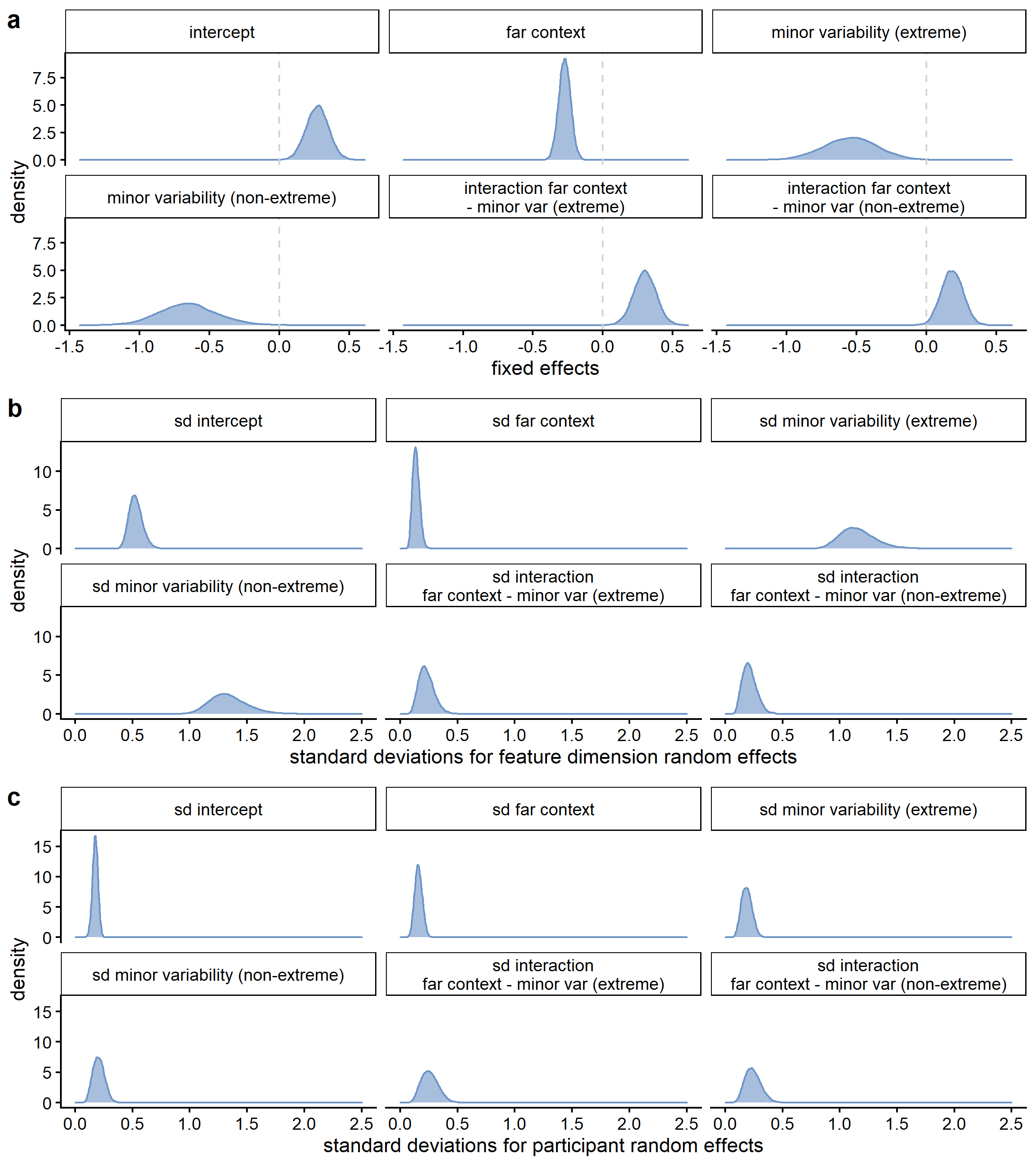
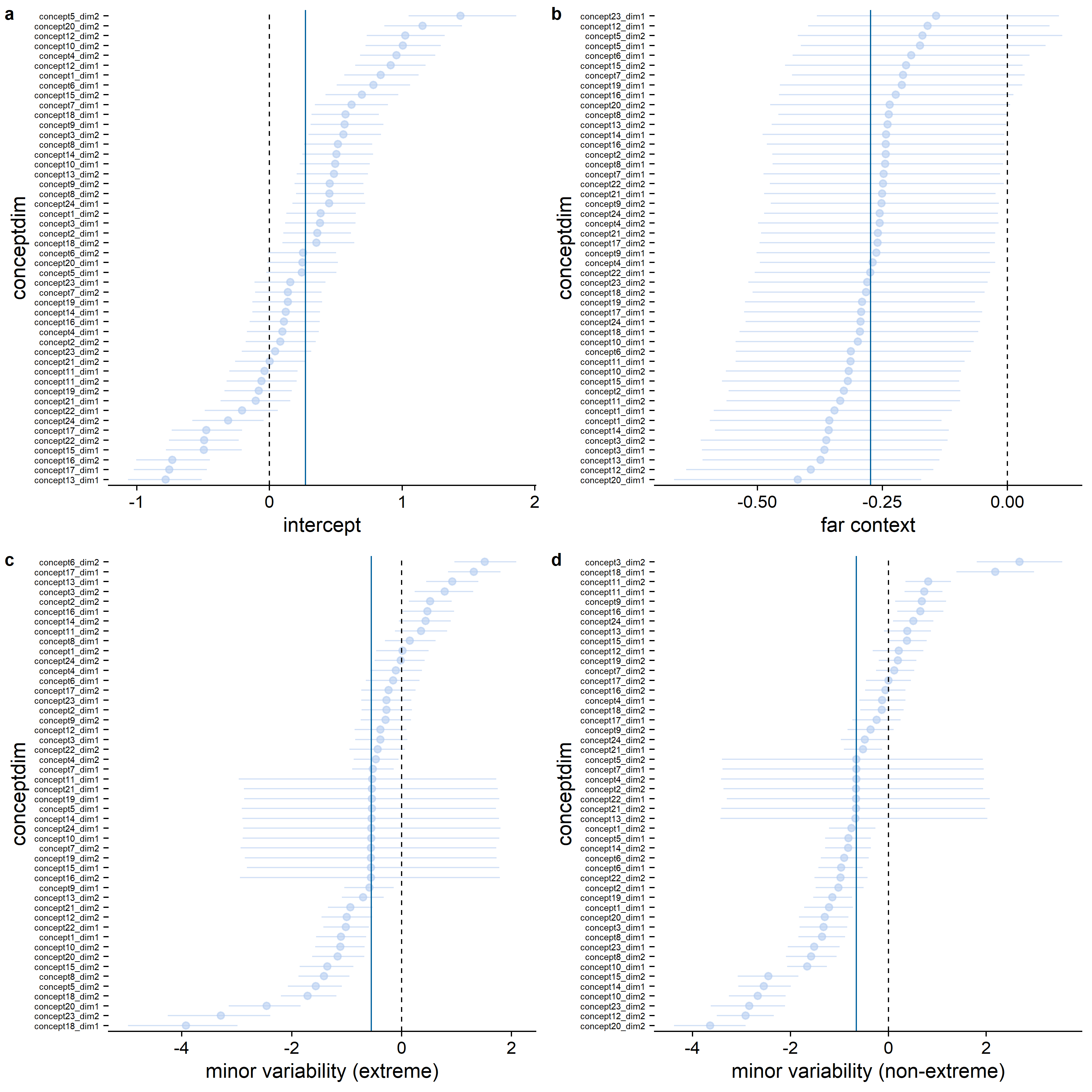
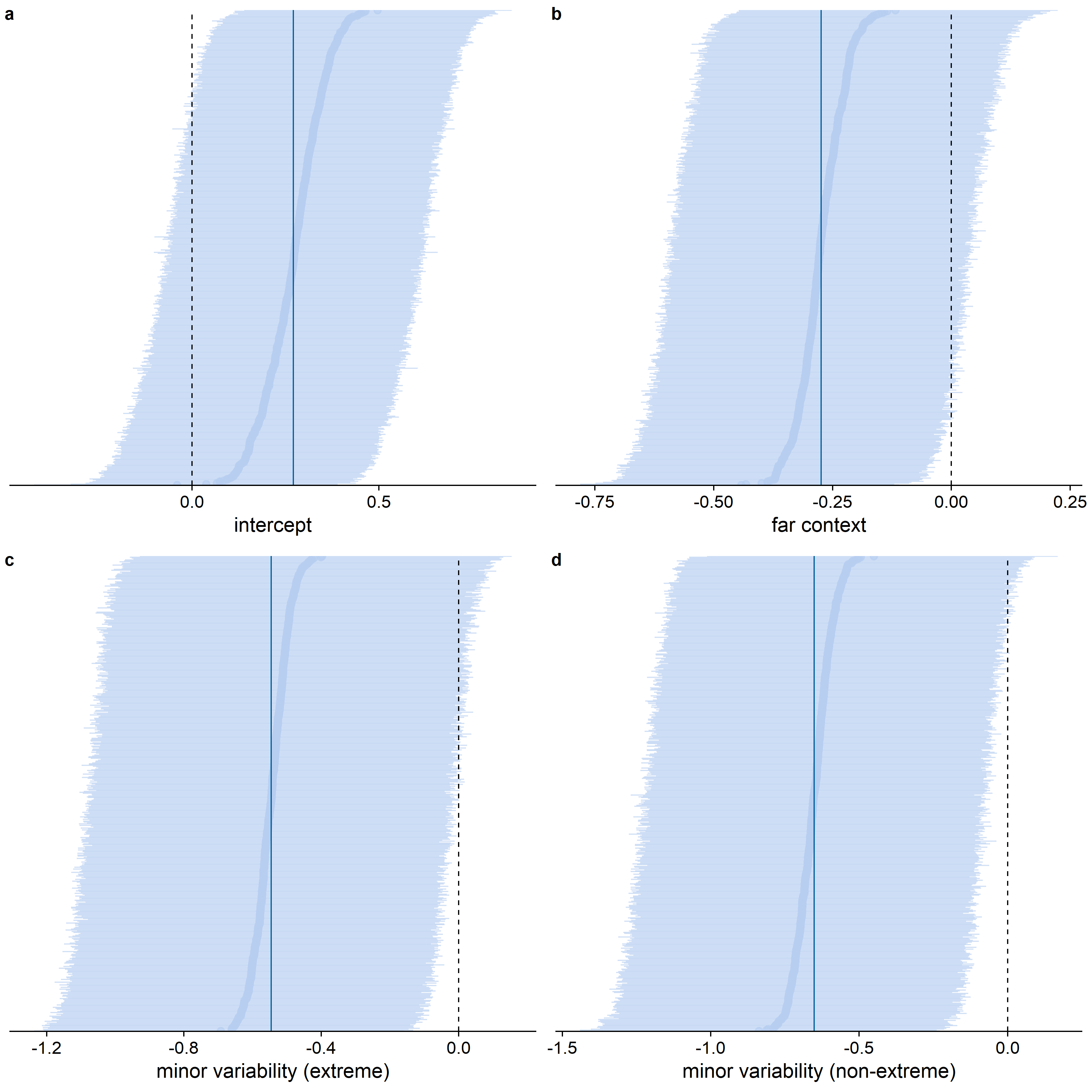
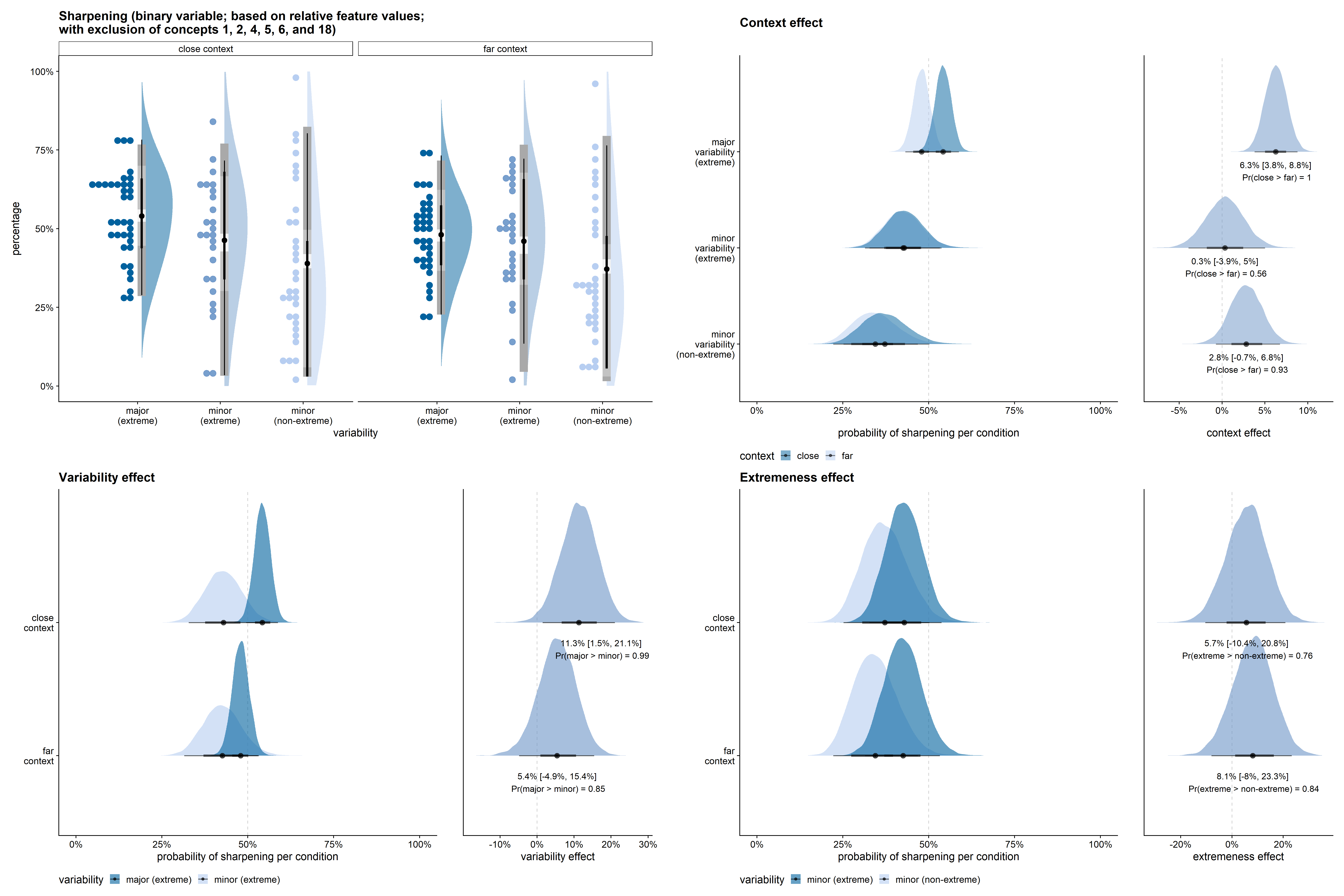
Figure D.4 shows the results for the equivalent qualitative model of sharpening based on the absolute rather than the relative feature values. Figure D.5 shows the results for the qualitative model of sharpening based on the relative feature values, but with exclusion of concepts 1, 2, 4, 5, 6, and 18.

Figure D.4: Results of the qualitative model of sharpening, defined as a drawn value equal to the target or more extreme, based on the absolute feature values.

Figure D.5: Results of the qualitative model of sharpening, defined as a drawn value equal to the target or more extreme, based on the relative feature values, with exclusion of concepts 1, 2, 4, 5, 6, and 18.

D.2.2 Qualitative results for the alternative interpretation of leveling and sharpening (binarized; relative values)

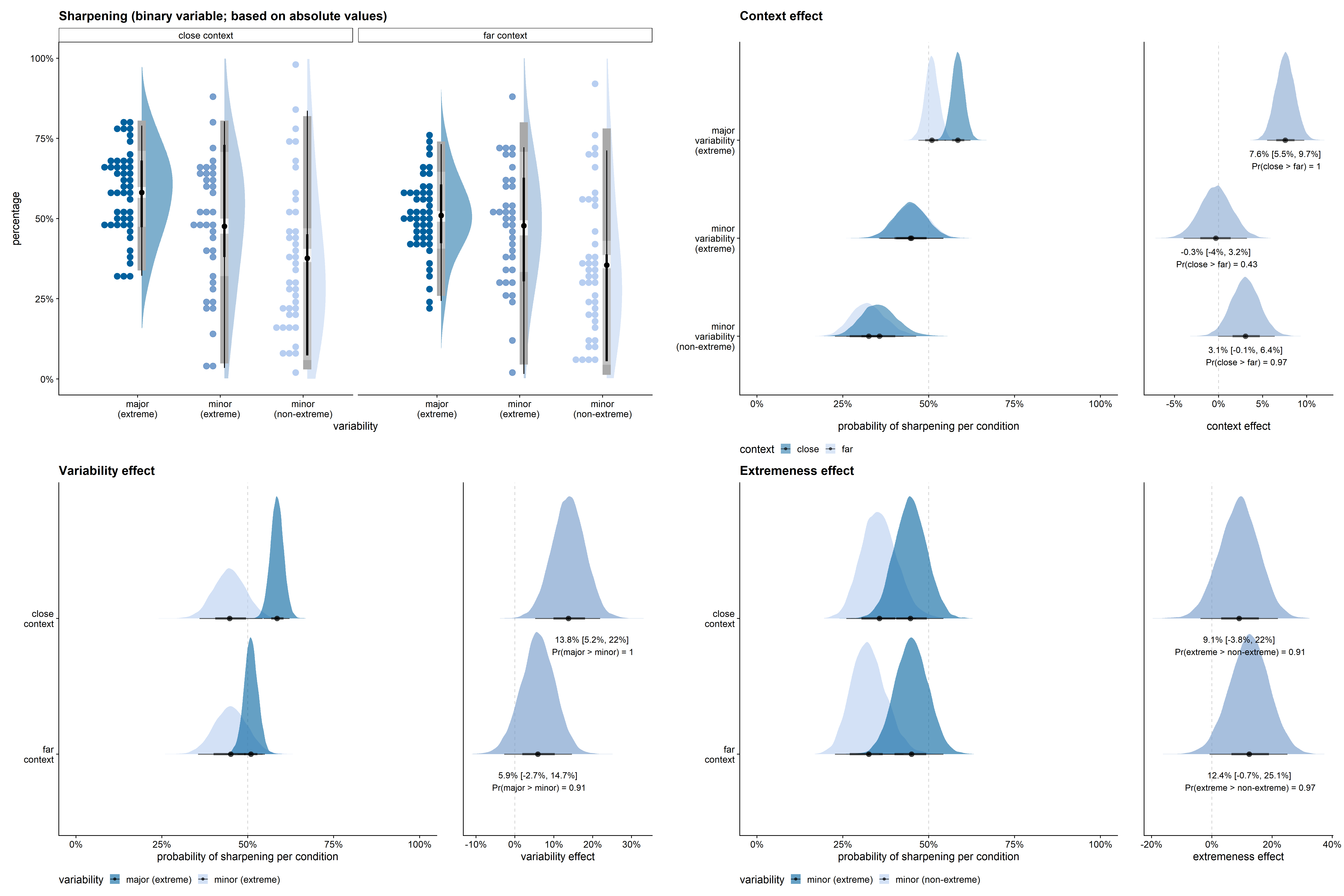
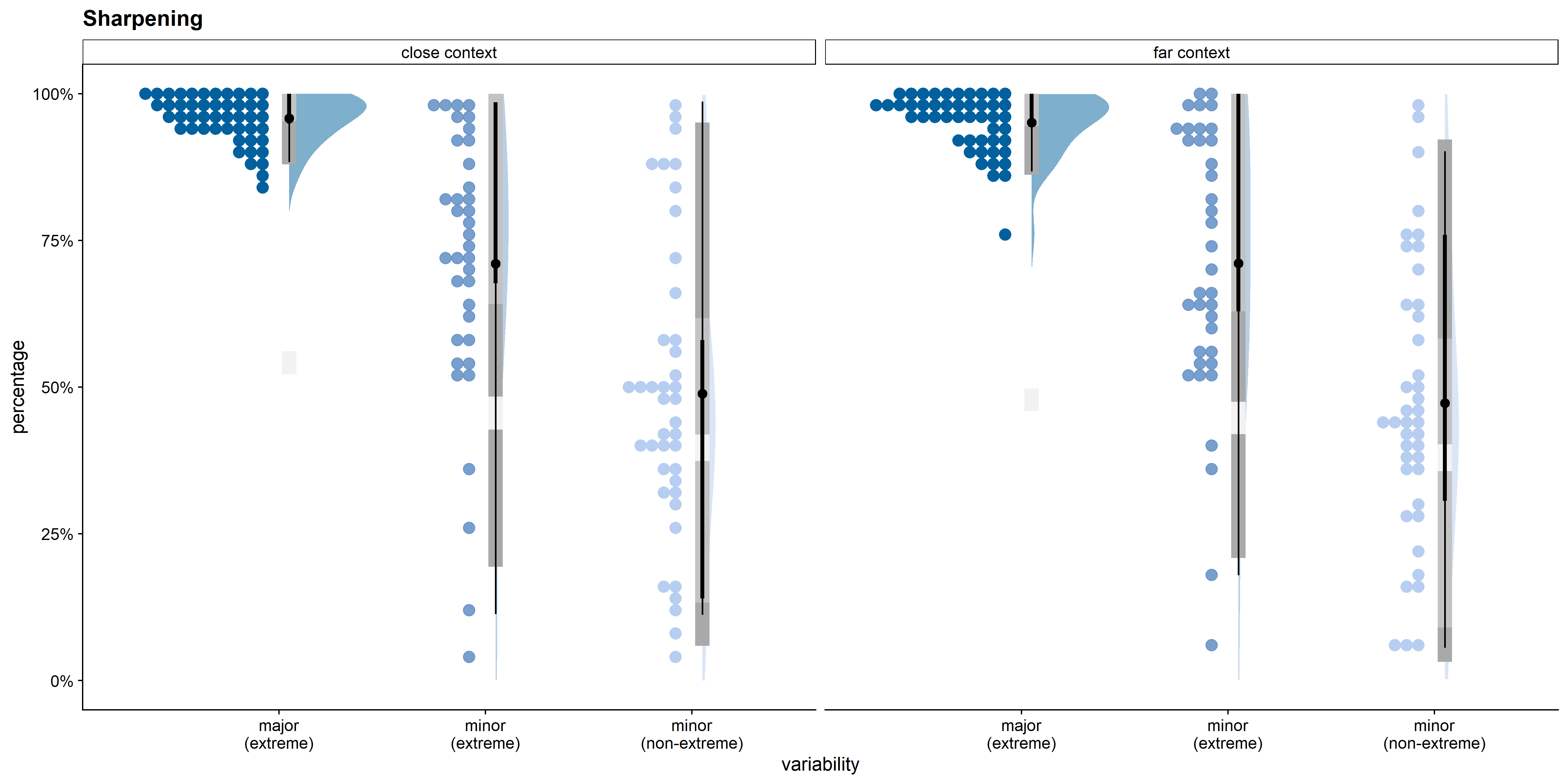
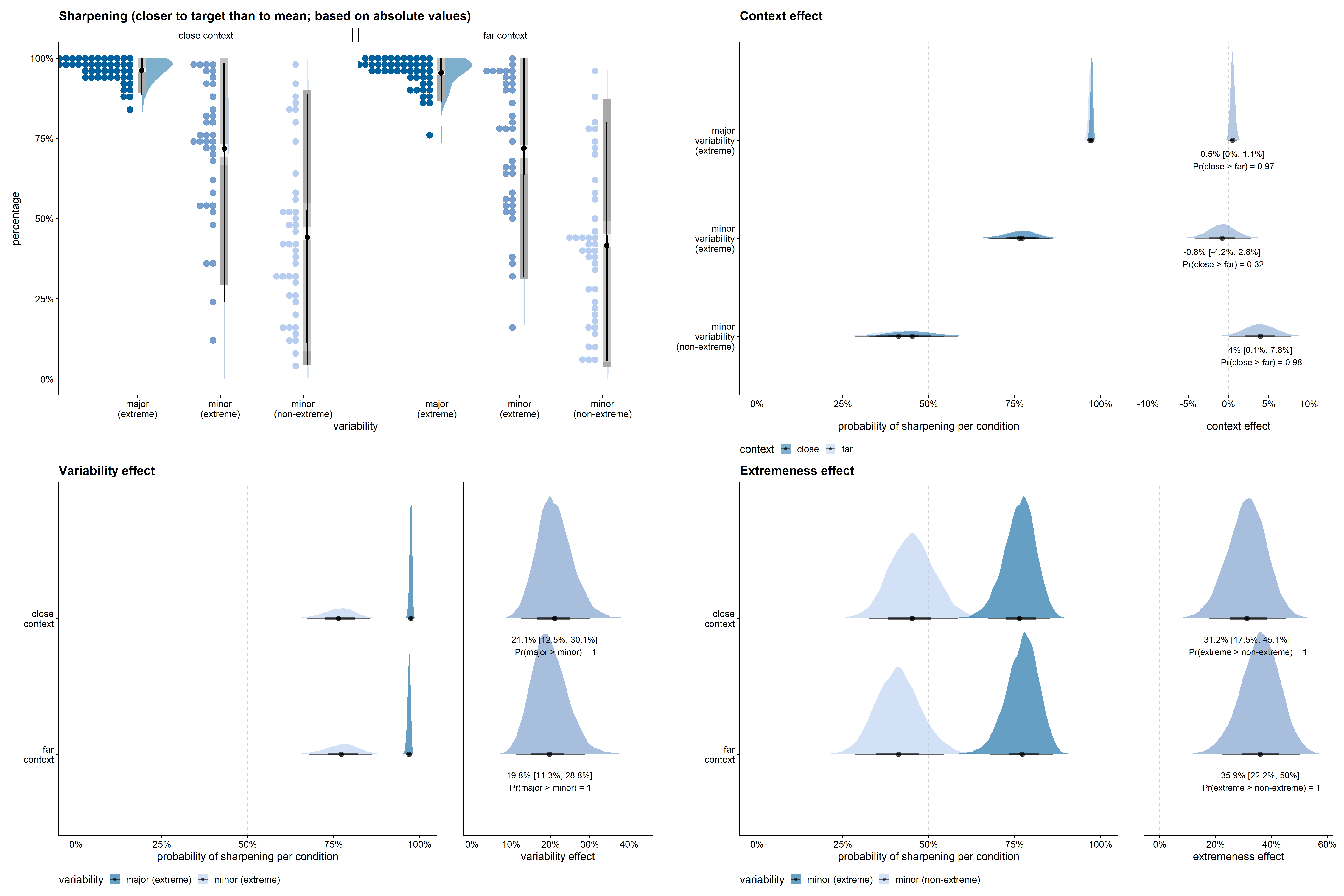
In Figure D.6, sharpening is defined as a drawn value closer to the target value than to the feature dimension’s mean. Defining sharpening in this manner, increased the differences between the three variability conditions and decreased the size of the context effect. The results stayed in the expected direction, however: sharpening was more likely for the major variability dimension than for the minor variability dimensions, and there was a tendency for sharpening to be more common in the close than in the far context. Furthermore, also using this definition of sharpening, there was much more variability in the percentage of sharpening across feature dimensions in the minor variability conditions than in the major variability condition.

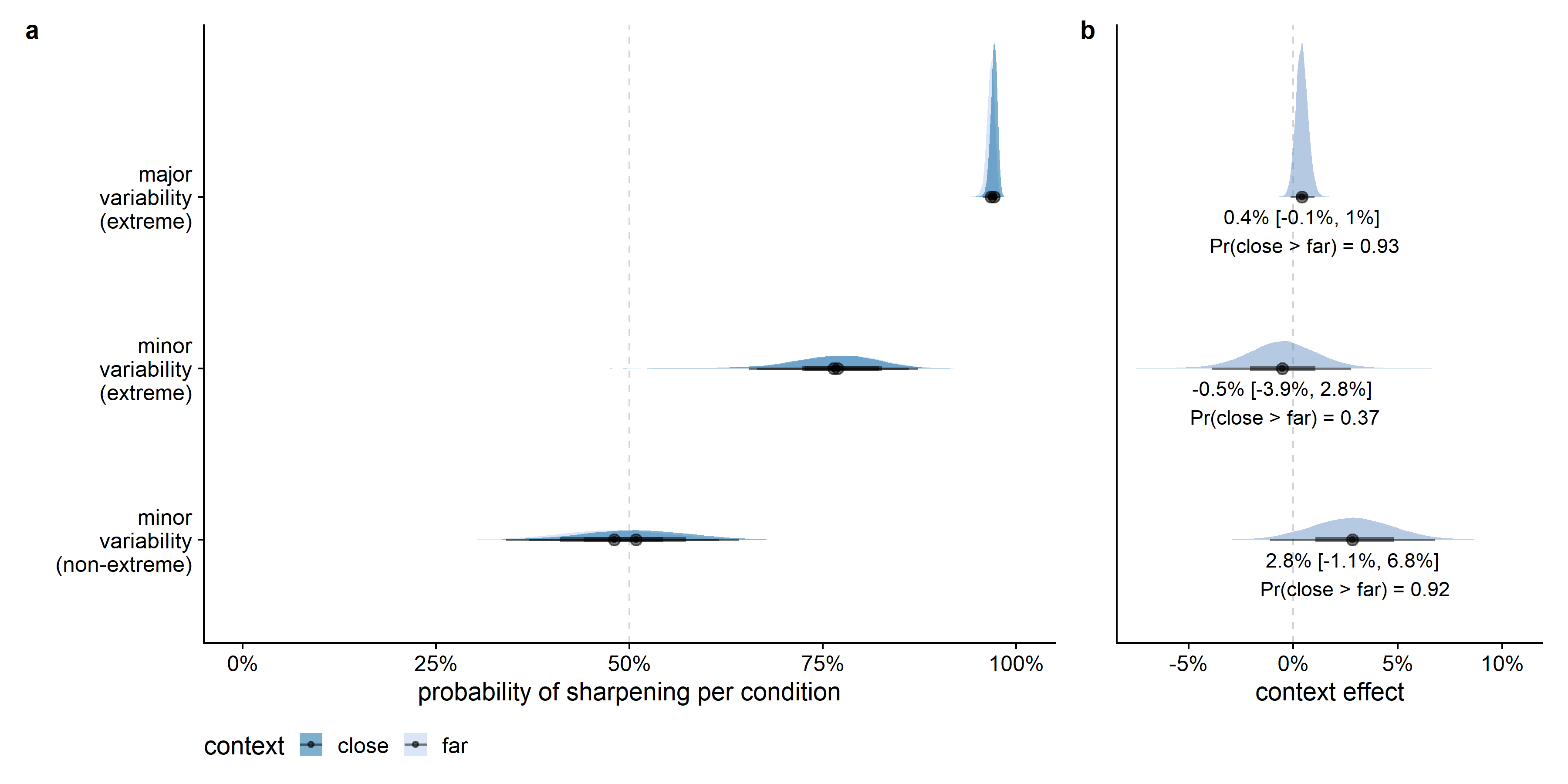
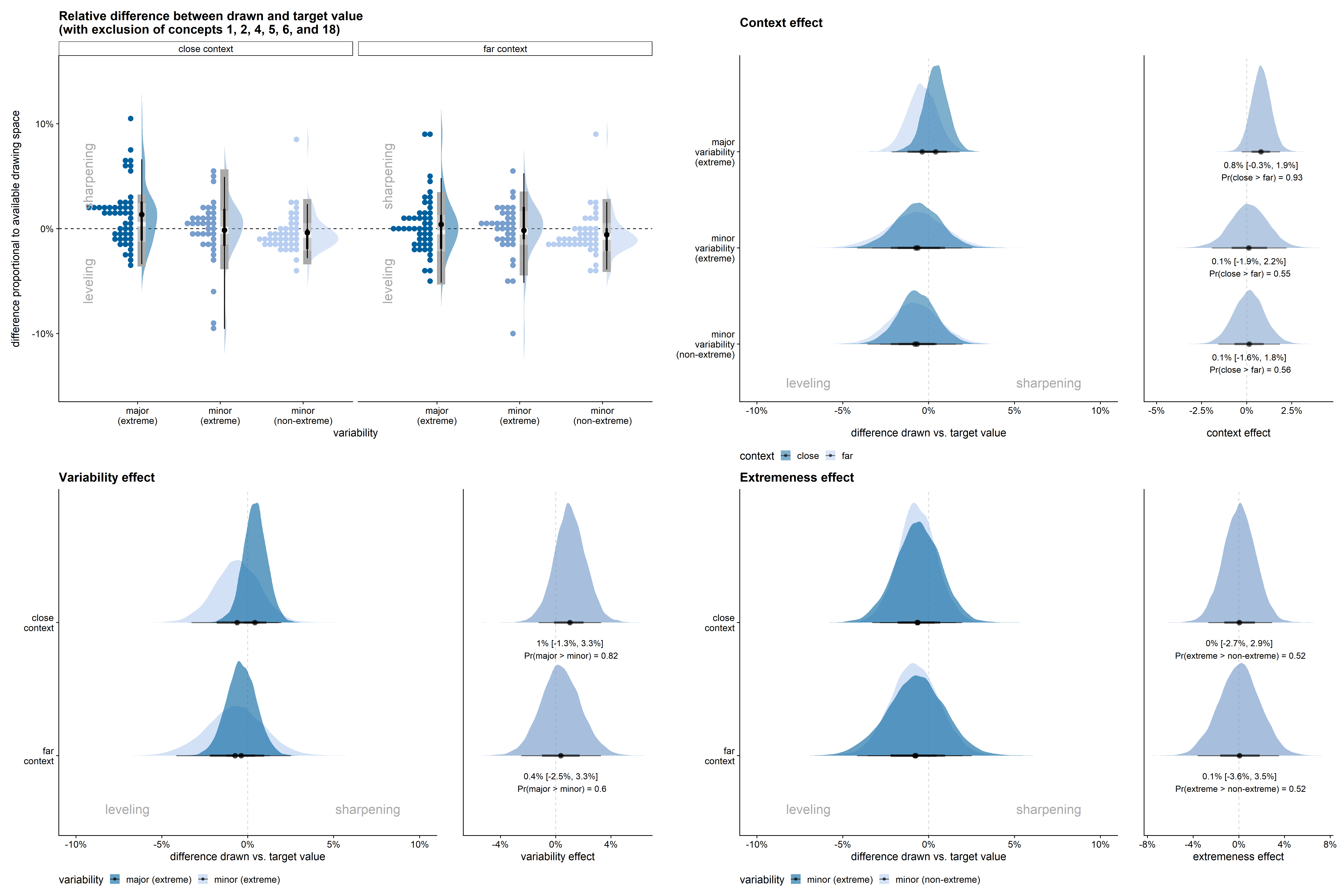
Figure D.7, Figure D.8, and Figure D.9 give the posterior estimates from the model per context and variability condition, and compare the slope strengths across conditions for the effects of context, variability, and extremeness, respectively. In the major variability condition, the posterior probability of the proportion of sharpening in the close context to be larger than in the far context was 93%. Even though the direction of the effect was highly probable in the expected direction, given this alternative definition of leveling and sharpening, the context effect was very limited in size (see Figure D.7).

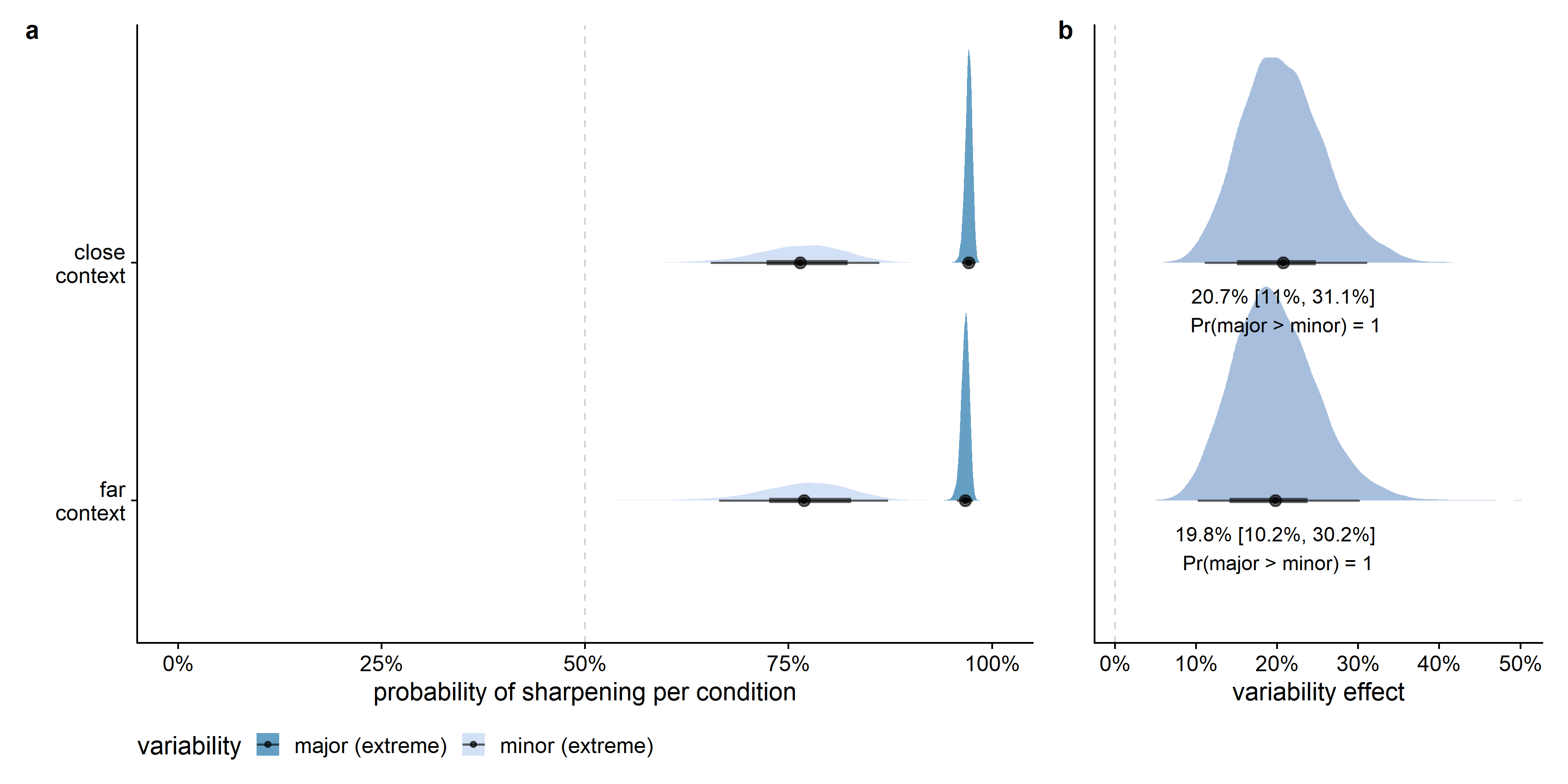
The effect of variability, however, was very large given this alternative interpretation of leveling and sharpening (see Figure D.8). In all posterior samples, the probability for an extreme value on the major feature dimension to be sharpened was larger than for an extreme value on a minor feature dimension. Given that the model is a good approximation of the data, the data provide evidence for a clear effect of variability in both the close and far context conditions.

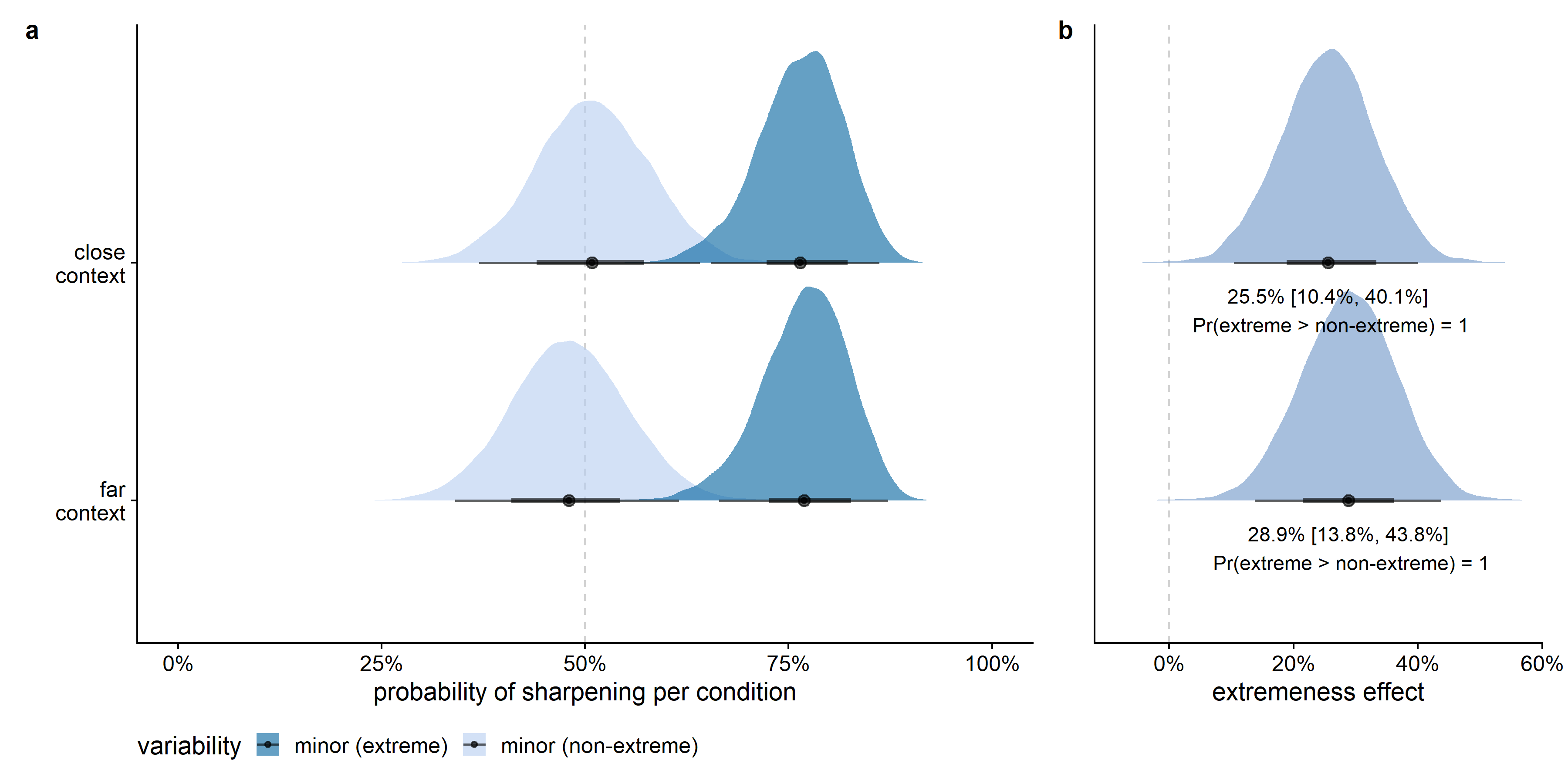
Also the effect of being one of the extrema on the feature dimension was very large given this alternative interpretation of leveling and sharpening (see Figure D.9). In all posterior samples, the probability for an extreme value on the minor feature dimension to be sharpened was larger than for a non-extreme value on a minor feature dimension. Given that the model is a good approximation of the data, the data provide evidence for a clear effect of extremeness in both the close and far context conditions.

Figure D.6: Distribution of percentage of times a feature dimension was sharpened, per context and variability condition, with feature dimensions as individual data points. The black point and intervals indicate mean and 66% and 95% highest density continuous intervals for the data distribution. The grey intervals indicate the 66% and 95% highest density continuous intervals for the posterior predictive distribution, based on the qualitative model of sharpening as binary variable using the relative feature values. In addition, the white interval indicates the 95% highest density continuous interval for the mean posterior prediction.

Figure D.7: (a) Posterior distribution for the probability of drawing a feature equal to the target value or more extreme, separately for each context and variability condition. (b) Estimated context effect in each variability condition. Mean, 66%, and 95% highest density continuous intervals are shown. The text also indicates the mean estimated difference with its 95% highest density continuous interval, as well as the posterior probability of the percentage of sharpening being higher in the close than in the far context, given a particular variability condition.

Figure D.8: (a) Posterior distribution for the probability of drawing a feature equal to the target value or more extreme, separately for the major (extreme) and minor (extreme) variability and context conditions. (b) Estimated variability effect in each context condition. Mean, 66%, and 95% highest density continuous intervals are shown. The text also indicates the mean estimated difference with its 95% highest density continuous interval, as well as the posterior probability of the percentage of sharpening being higher in case the feature exhibits major compared to minor variability, given a particular context condition.

Figure D.9: (a) Posterior distribution for the probability of drawing a feature equal to the target value or more extreme, separately for the minor (extreme) and minor (non-extreme) variability and context conditions. (b) Estimated variability effect in each context condition. Mean, 66%, and 95% highest density continuous intervals are shown. The text also indicates the mean estimated difference with its 95% highest density continuous interval, as well as the posterior probability of the percentage of sharpening being higher in case the feature value is one of the extrema on the dimension, given a particular context condition.

Just as in the models using the other interpretations of leveling and sharpening, the estimated variability between feature dimensions was larger for the differences between the variability and extremeness conditions than for the context effect (see Figure D.10), and the estimated variability between feature dimensions was higher than the estimated variability between participants, which is potentially also a consequence of the limited number of data points per participant in comparison to the number of data points per feature dimension.

Figure D.10: Posterior distributions of fixed effects and standard deviations of random effects for concept and dimension combined, for the qualitative model, using the alternative interpretation of sharpening as a drawn value closer to the target value than to the mean value on the dimension (binarized; based on relative feature values).

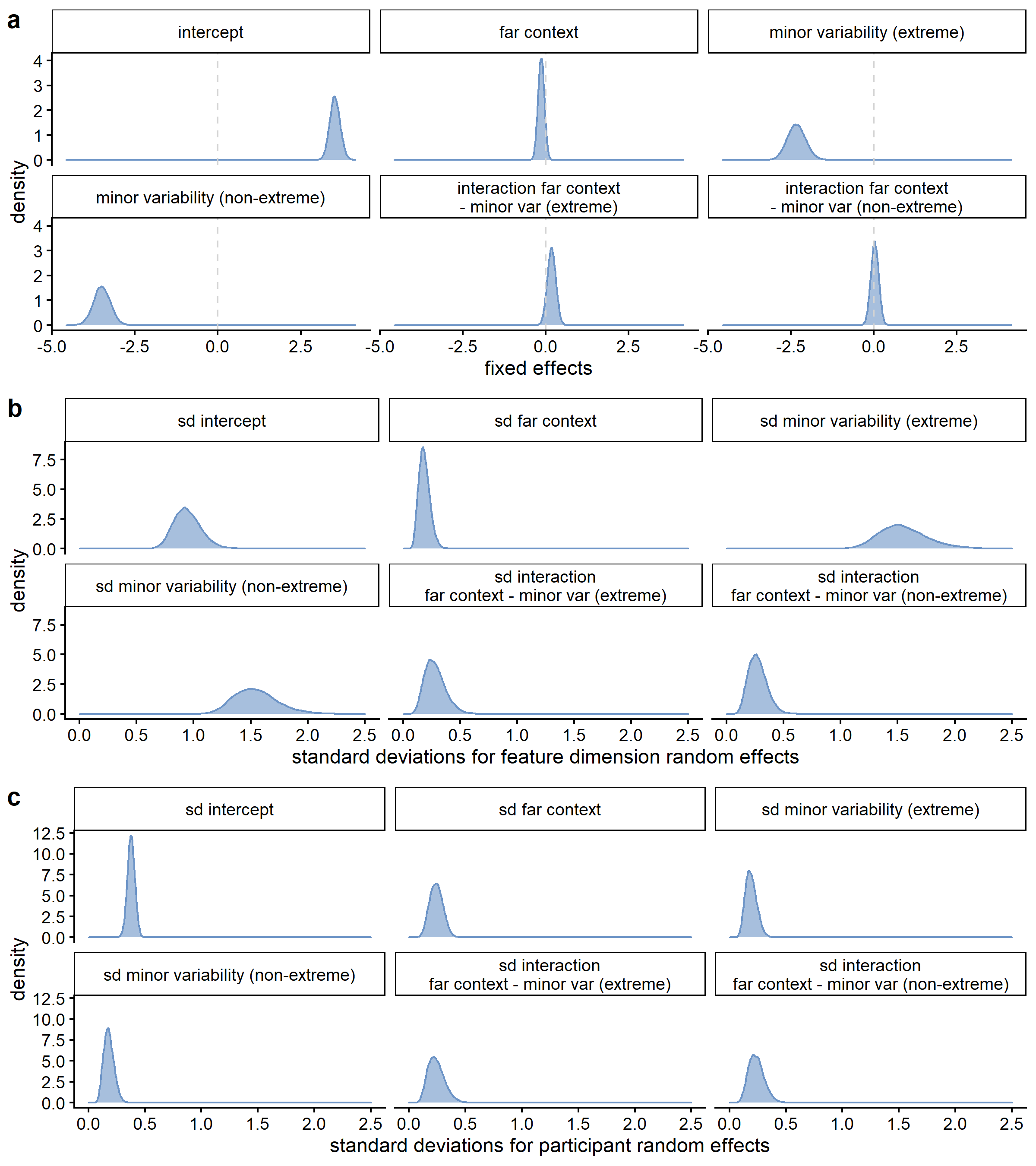
Figure D.11 shows the results for the equivalent qualitative model of sharpening based on the absolute rather than the relative feature values.

Figure D.11: Results of the qualitative model of sharpening, defined as a drawn value closer to the target than to the mean, based on the absolute feature values.

D.2.3 Additional quantitative results

When inspecting the standard deviations for the feature dimension random effects (see Figure D.12), the estimated variability between feature dimensions was slightly larger for the differences between the variability conditions than for the context effect, but the difference in variability seemed less outspoken than in the qualitative analysis (see also Figure D.13). As in the other models, the estimated variability between feature dimensions was higher than the estimated variability between participants (see also Figure D.14).

Figure D.12: Posterior distributions of fixed effects and standard deviations of random effects for concept and dimension combined, for the quantitative model (based on relative feature values).

Figure D.13: Slopes for the intercept, the effect of context, the effect of a minor extreme feature value compared to a major extreme feature value, and the effect of a minor non-extreme feature value compared to a major extreme feature value on drawing a feature equal to the target value or more extreme, per feature dimension. Mean and 95% highest density continuous intervals are shown. The blue line indicates the average mean value across feature dimensions. The dashed black line indicates a value of zero. Note. The very wide intervals for some feature dimensions are the consequence of those feature dimensions not being present in the relevant condition, e.g., no minor variability (extreme) condition for that feature dimension.

Figure D.14: Slopes for the intercept, the effect of context, the effect of a minor extreme feature value compared to a major extreme feature value, and the effect of a minor non-extreme feature value compared to a major extreme feature value on drawing a feature equal to the target value or more extreme, per participant. Mean and 95% highest density continuous intervals are shown. The blue line indicates the average mean value across participants. The dashed black line indicates a value of zero.

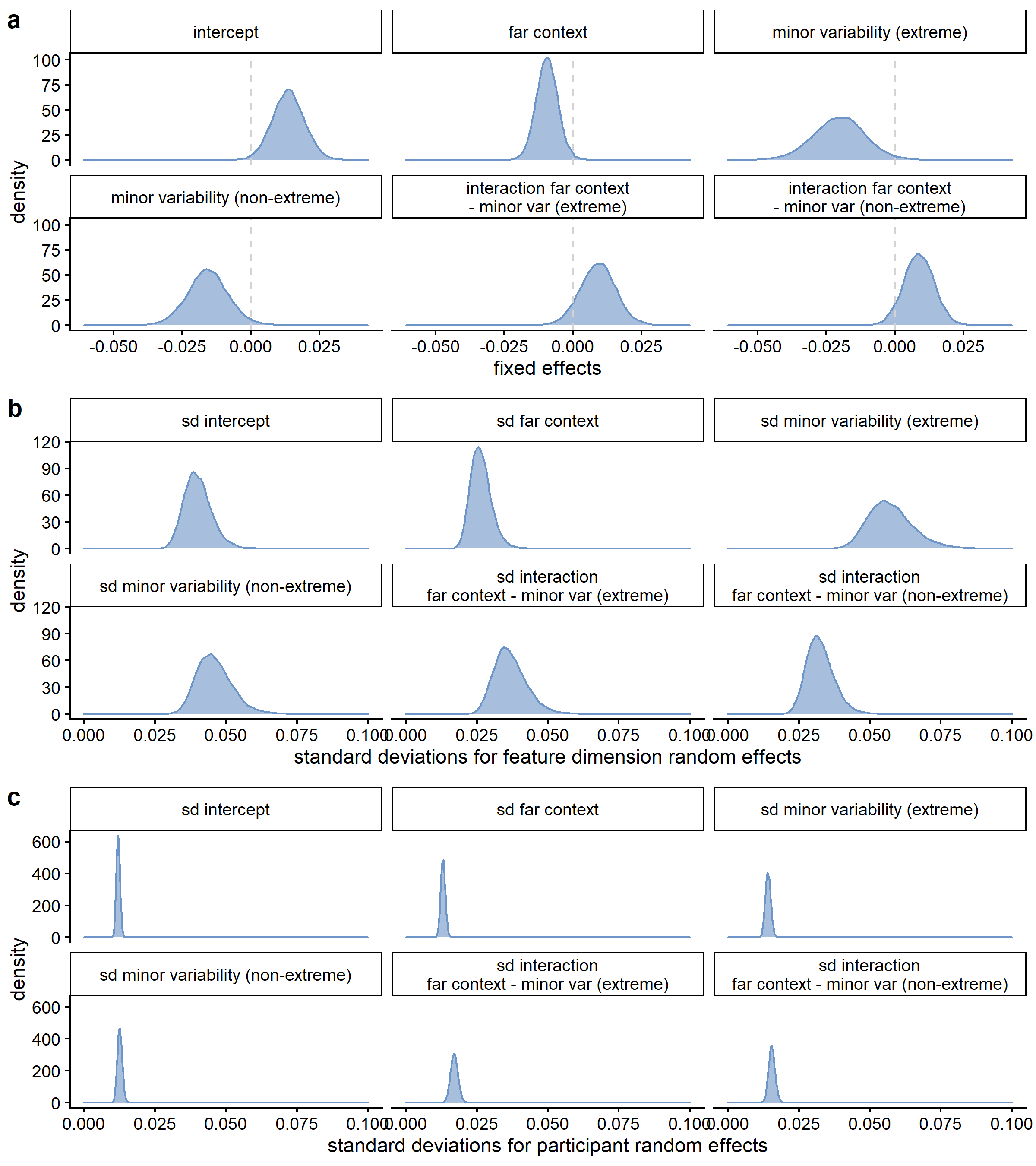
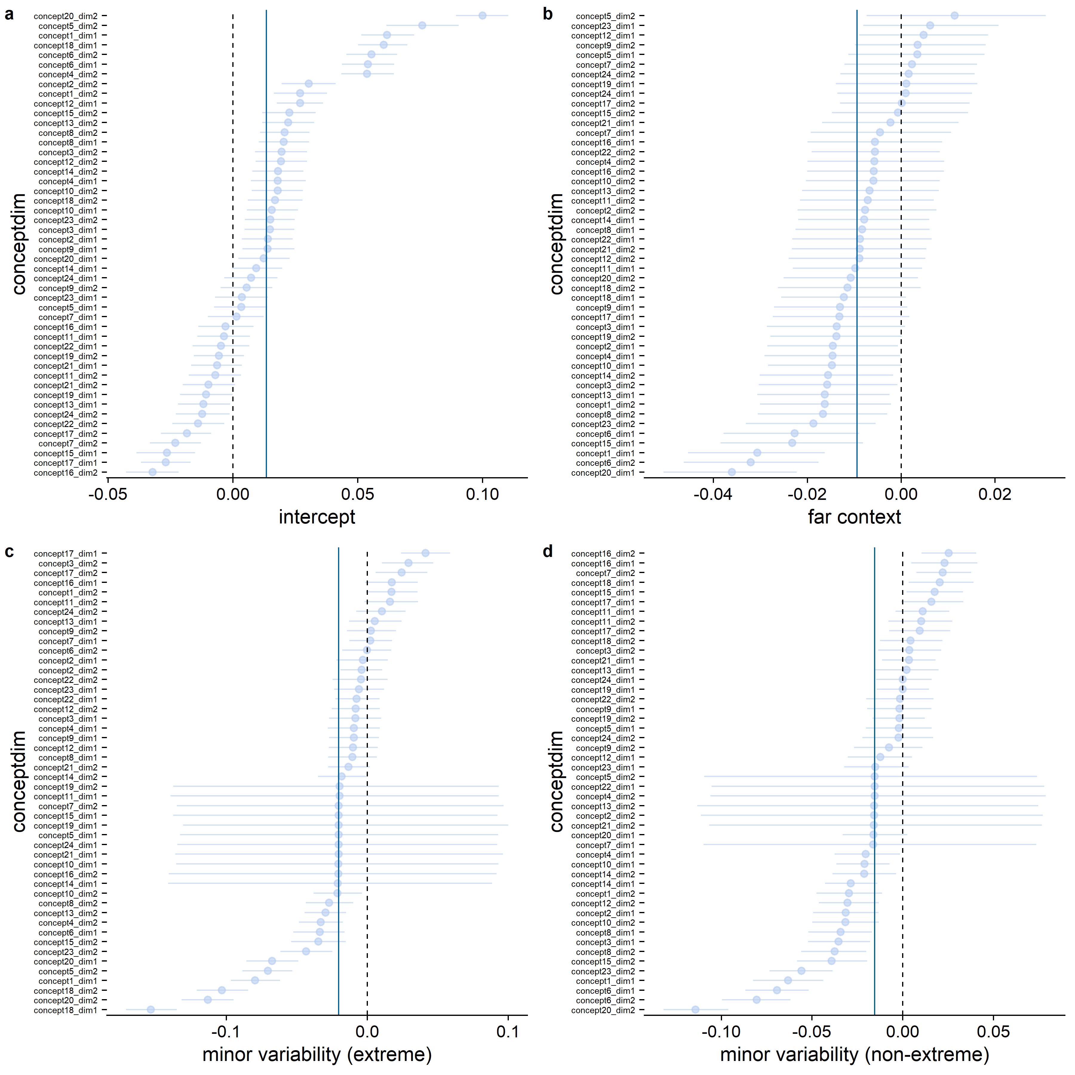
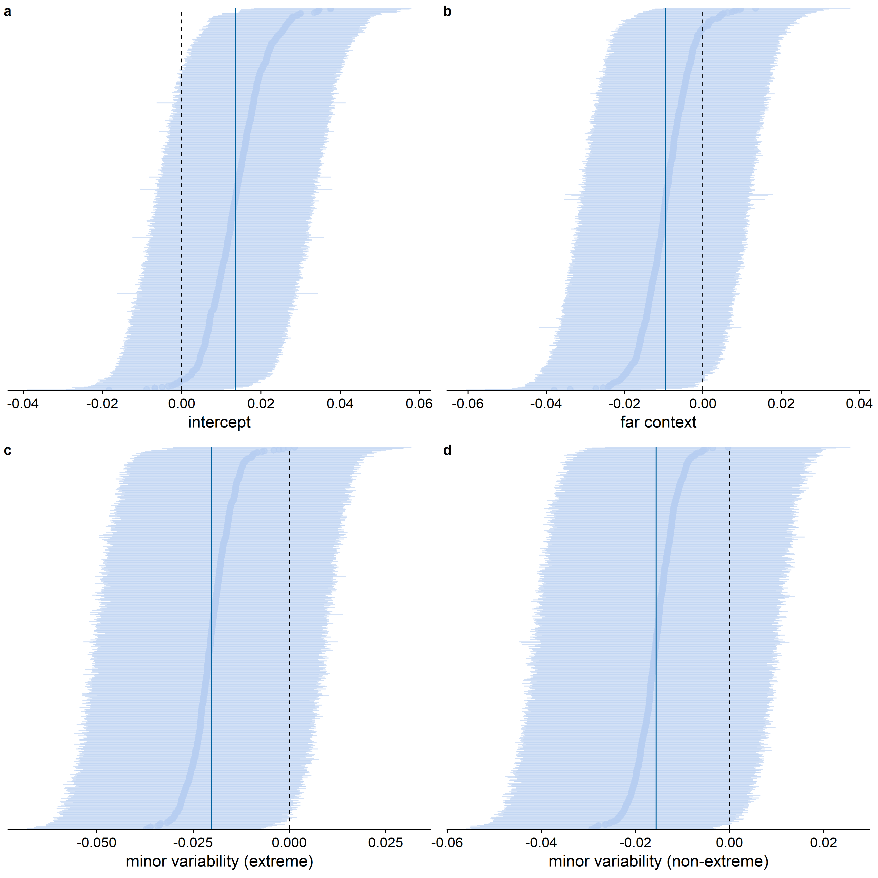
Figure D.15 shows the results for the quantitative model of sharpening based on the relative feature values, but with exclusion of concepts 1, 2, 4, 5, 6, and 18.

Figure D.15: Results of the quantitative model of sharpening, defined as a drawn value equal to the target or more extreme, based on the relative feature values, with exclusion of concepts 1, 2, 4, 5, 6, and 18.

D.3 Supplemental videos

In the HTML version of this Appendix, you can find screen recordings of some components that were part of this study (cf. Figure D.16).

Instructions and informed consent

Resizing procedure

Demographics questions

Interface instructions

Practice drawing

Drawing task

Figure D.16: Screen recordings of some components that were part of this study.

Aust, F., & Barth, M. (2022). papaja: Prepare reproducible APA journal articles with R Markdown. https://github.com/crsh/papaja

Barth, M. (2022). tinylabels: Lightweight variable labels. https://cran.r-project.org/package=tinylabels

Bürkner, P.-C. (2017). brms: An R package for Bayesian multilevel models using Stan. Journal of Statistical Software, 80(1), 1–28. https://doi.org/10.18637/jss.v080.i01

Bürkner, P.-C. (2018). Advanced Bayesian multilevel modeling with the R package brms. The R Journal, 10(1), 395–411. https://doi.org/10.32614/RJ-2018-017

Bürkner, P.-C. (2021). Bayesian item response modeling in R with brms and Stan. Journal of Statistical Software, 100(5), 1–54. https://doi.org/10.18637/jss.v100.i05

Cheng, J., Sievert, C., Schloerke, B., Chang, W., Xie, Y., & Allen, J. (2021). Htmltools: Tools for HTML. https://CRAN.R-project.org/package=htmltools

Eddelbuettel, D., & Balamuta, J. J. (2018). Extending extitR with extitC++: A Brief Introduction to extitRcpp. The American Statistician, 72(1), 28–36. https://doi.org/10.1080/00031305.2017.1375990

Eddelbuettel, D., & François, R. (2011). Rcpp: Seamless R and C++ integration. Journal of Statistical Software, 40(8), 1–18. https://doi.org/10.18637/jss.v040.i08

Henry, L., & Wickham, H. (2020). Purrr: Functional programming tools. https://CRAN.R-project.org/package=purrr

Henry, L., Wickham, H., & Chang, W. (2020). Ggstance: Horizontal ’ggplot2’ components. https://CRAN.R-project.org/package=ggstance

Kay, M. (2021a). ggdist: Visualizations of distributions and uncertainty. https://doi.org/10.5281/zenodo.3879620

Kay, M. (2021b). tidybayes: Tidy data and geoms for Bayesian models. https://doi.org/10.5281/zenodo.1308151

Müller, K. (2020). Here: A simpler way to find your files. https://CRAN.R-project.org/package=here

Müller, K., & Wickham, H. (2022). Tibble: Simple data frames. https://CRAN.R-project.org/package=tibble

Pedersen, T. L. (2022). Patchwork: The composer of plots. https://CRAN.R-project.org/package=patchwork

R Core Team. (2021). R: A language and environment for statistical computing. R Foundation for Statistical Computing. https://www.R-project.org/

Stan Development Team. (2020a). RStan: The R interface to Stan. http://mc-stan.org/

Stan Development Team. (2020b). StanHeaders: Headers for the R interface to Stan. https://mc-stan.org/

Tiedemann, F. (2020). Gghalves: Compose half-half plots using your favourite geoms. https://CRAN.R-project.org/package=gghalves

Wickham, H. (2016). ggplot2: Elegant graphics for data analysis. Springer-Verlag New York. https://ggplot2.tidyverse.org

Wickham, H. (2019). Stringr: Simple, consistent wrappers for common string operations. https://CRAN.R-project.org/package=stringr

Wickham, H. (2022). Forcats: Tools for working with categorical variables (factors). https://CRAN.R-project.org/package=forcats

Wickham, H., Averick, M., Bryan, J., Chang, W., McGowan, L. D., François, R., Grolemund, G., Hayes, A., Henry, L., Hester, J., Kuhn, M., Pedersen, T. L., Miller, E., Bache, S. M., Müller, K., Ooms, J., Robinson, D., Seidel, D. P., Spinu, V., … Yutani, H. (2019). Welcome to the tidyverse. Journal of Open Source Software, 4(43), 1686. https://doi.org/10.21105/joss.01686

Wickham, H., François, R., Henry, L., & Müller, K. (2022). Dplyr: A grammar of data manipulation. https://CRAN.R-project.org/package=dplyr

Wickham, H., & Girlich, M. (2022). Tidyr: Tidy messy data. https://CRAN.R-project.org/package=tidyr

Wickham, H., Hester, J., & Bryan, J. (2022). Readr: Read rectangular text data. https://CRAN.R-project.org/package=readr

Wilke, C. O. (2020). Cowplot: Streamlined plot theme and plot annotations for ’ggplot2’. https://CRAN.R-project.org/package=cowplot

Xie, Y. (2015). Dynamic documents with R and knitr (2nd ed.). Chapman; Hall/CRC. https://yihui.org/knitr/

---

1. Due to rounding errors, the size of the steps between the different values on a feature dimension was not always exactly equal, especially for the feature dimensions with minor variability. In addition, when constructing the stimuli, some errors were made in the minimum or maximum value for the dimension with minor variability for designs 5 (maximum value dimension 1 in series B 28.25 instead of 28.75), 16 (minimum value dimension 1 in series B 30 instead of 31.2), and 22 (minimum value dimension 1 in series B 23.8 instead of 21.2 and maximum value dimension 1 in series B 31.2 instead of 28.8).

2. For designs 1, 2, and 6, one of the feature dimensions was bidirectional, which required the step size to be added at both sides of the figure. Therefore, in these designs, the smallest steps were one out of two or one out of eight of the largest steps available concurrently for the other feature dimension in the figure. When comparing major and minor variability for the same feature dimension across the A and B series, the ratio of one out of four is correct.

3. One downside of this rescaling procedure is that the height and/or width of the two drawn shapes becomes dependent, potentially indirectly leading to dependent feature values on both dimensions. The rescaling can also lead to feature values relative to the available drawing space that are smaller than -1 or larger than 1. We therefore also conducted the analyses with exclusion of these six designs, which led to slightly smaller but similar qualitative and quantitative results as presented in the main text (see Figure D.5 and Figure D.15).